
Implemented Deep Learning Projects
Repo for all the projects ( vertical post)…
Welcome back peeps.
Since we are now focusing on our goals for 2023 — new vertical series than horizontal ( means you will find all the contents of the series in one post and projects in second than developing/extending it to new posts every time). So, keep checking this post every day to see new projects.
Prerequisite to these projects —
Complete 60 days of Data Science and Machine Learning before starting this series ( link below) —
Projects Videos —
All the projects, data structures, SQL, algorithms, system design, Data Science and ML , Data Analytics, Data Engineering, , Implemented Data Science and ML projects, Implemented Data Engineering Projects, Implemented Deep Learning Projects, Implemented Machine Learning Ops Projects, Implemented Time Series Analysis and Forecasting Projects, Implemented Applied Machine Learning Projects, Implemented Tensorflow and Keras Projects, Implemented PyTorch Projects, Implemented Scikit Learn Projects, Implemented Big Data Projects, Implemented Cloud Machine Learning Projects, Implemented Neural Networks Projects, Implemented OpenCV Projects,Complete ML Research Papers Summarized, Implemented Data Analytics projects, Implemented Data Visualization Projects, Implemented Data Mining Projects, Implemented Natural Leaning Processing Projects, MLOps and Deep Learning, Applied Machine Learning with Projects Series, PyTorch with Projects Series, Tensorflow and Keras with Projects Series, Scikit Learn Series with Projects, Time Series Analysis and Forecasting with Projects Series, ML System Design Case Studies Series videos will be published on our youtube channel ( just launched).
Subscribe today!
Tech Newsletter —
If you are interested, you can join my newsletter through which I send tech interview tips, techniques, patterns, hacks — Software Development, ML, Data Science, Startups and Technology projects to more than 35K readers. You can subscribe to Ignito:
Let’s dive in!
Deep learning is a subfield of machine learning that is inspired by the structure and function of the human brain. It involves the use of neural networks, which are a type of model made up of layers of interconnected nodes, called neurons.
These networks are trained using a large dataset of labeled examples, and can be used for a wide range of tasks such as image recognition, speech recognition, natural language processing, and more.
Deep learning models consist of multiple layers of neurons, which allows them to learn increasingly complex representations of the data. The most common types of deep learning models are feedforward neural networks, convolutional neural networks, and recurrent neural networks.
- Feedforward neural networks are the simplest type of deep learning models, where the data flows through the network from input to output, without looping back.
- Convolutional Neural Networks (CNN) are specially designed for image processing, it is a feedforward neural network where the layers are designed to process the spatial structure of images, such as edges, shapes, and textures.
- Recurrent Neural Networks (RNN) are designed to process sequential data such as time series, audio, and text. These networks include feedback connections, which allow them to maintain a hidden state that captures information about previous inputs.
Deep learning models are trained using a variant of stochastic gradient descent (SGD) called backpropagation. The model is trained on a large dataset of labeled examples and the weights of the neurons are adjusted during training to minimize the error between the model’s predictions and the true labels.
Deep learning models have been shown to be highly effective for a wide range of tasks, and have been adopted in many applications such as image classification, speech recognition, natural language processing, and more. They have also been used to achieve state-of-the-art performance on a wide range of benchmarks and competitions.
This post will house all the Deep learning projects related to the topics below-
Neural Networks
Convolutional Neural Networks
Recurrent Neural Networks
Tensorflow
Autoencoders
Generative Adversarial Networks
Attention and Transformers
Graph Neural Networks
Natural Language Processing
Federated learning
First we will cover above mentioned topics in detail and their implementation before starting the projects —
Neural network
Neural networks are like a big team of helpers that work together to solve problems. Just like you have different friends who are good at different things, a neural network has lots of little helpers called “neurons” that each know how to do their own small job.
- When you want the neural network to solve a problem, you give it some information to start with. Each neuron looks at that information and decides whether it’s helpful or not. If it’s helpful, the neuron will send a message to other neurons that it’s connected to. Those neurons will then look at the information and decide whether it’s helpful too, and they might pass the message along to other neurons.
- Eventually, all of the neurons work together to come up with an answer to the problem. It’s kind of like a big group of friends working together to solve a puzzle. Each friend has their own strengths, and by working together they can solve the puzzle much faster and more easily than if they tried to do it alone.
So that’s basically what a neural network is — a big group of little helpers working together to solve problems!
A neural network is a type of machine learning model inspired by the structure and function of the human brain. The main building blocks of a neural network are artificial neurons, also called nodes, which are organized into layers.
Neural networks can be used for a wide range of tasks, including image classification, language translation, and even playing games.
Implementation of a neural network in Python using the popular deep learning library TensorFlow:
import tensorflow as tf# Define the input layer
input_layer = tf.keras.layers.Input(shape=(10,))# Define a hidden layer with 64 nodes and activation function ReLU
hidden_layer = tf.keras.layers.Dense(64, activation='relu')(input_layer)# Define the output layer with 10 nodes and activation function softmax
output_layer = tf.keras.layers.Dense(10, activation='softmax')(hidden_layer)# Create a model with the input, hidden, and output layers
model = tf.keras.models.Model(inputs=input_layer, outputs=output_layer)# Compile the model using categorical cross-entropy loss and the Adam optimizer
model.compile(loss='categorical_crossentropy', optimizer='adam', metrics=['accuracy'])# Train the model on a dataset
model.fit(X_train, y_train, epochs=10, batch_size=32)# Evaluate the model on a test dataset
test_loss, test_acc = model.evaluate(X_test, y_test)
print('Test accuracy:', test_acc)In this implementation, we use the Input class to define the input layer with a shape of (10,), meaning it accepts a batch of 10-dimensional vectors. The Dense class is used to define dense, fully-connected layers, where each node in a layer is connected to all nodes in the previous layer. The relu activation function is used in the hidden layer to introduce non-linearity, and the softmax activation function is used in the output layer to produce a probability distribution over the possible classes. The model is then compiled with categorical cross-entropy loss and the Adam optimizer, and trained on a dataset using the fit method. Finally, the model is evaluated on a test dataset to measure its accuracy.
Types of Neural Networks —
There are several types of neural networks, each with their own strengths and weaknesses, that can be used for various tasks in deep learning. Some of the most common types are:
- Feedforward Neural Network: This is a simple type of neural network in which the data flows in one direction, from the input layer through the hidden layer(s) and finally to the output layer. It is used for tasks such as image classification and language translation.
import tensorflow as tf# Define the input layer
input_layer = tf.keras.layers.Input(shape=(10,))# Define a hidden layer with 64 nodes and activation function ReLU
hidden_layer = tf.keras.layers.Dense(64, activation='relu')(input_layer)# Define the output layer with 10 nodes and activation function softmax
output_layer = tf.keras.layers.Dense(10, activation='softmax')(hidden_layer)# Create a model with the input, hidden, and output layers
model = tf.keras.models.Model(inputs=input_layer, outputs=output_layer)# Compile the model using categorical cross-entropy loss and the Adam optimizer
model.compile(loss='categorical_crossentropy', optimizer='adam', metrics=['accuracy'])# Train the model on a dataset
model.fit(X_train, y_train, epochs=10, batch_size=32)# Evaluate the model on a test dataset
test_loss, test_acc = model.evaluate(X_test, y_test)
print('Test accuracy:', test_acc)- Convolutional Neural Network (CNN): This type of neural network is used for image classification and other computer vision tasks. It is designed to automatically and adaptively learn spatial hierarchies of features from input dataset through multiple levels of convolution and pooling operations.
Implement a basic CNN using Keras:
from tensorflow.keras.models import Sequential
from tensorflow.keras.layers import Conv2D, MaxPooling2D, Flatten, Dense

# Define the model architecture
model = Sequential()
model.add(Conv2D(32, (3, 3), activation='relu', input_shape=(28, 28, 1)))
model.add(MaxPooling2D((2, 2)))
model.add(Conv2D(64, (3, 3), activation='relu'))
model.add(MaxPooling2D((2, 2)))
model.add(Conv2D(64, (3, 3), activation='relu'))
model.add(Flatten())
model.add(Dense(64, activation='relu'))
model.add(Dense(10, activation='softmax'))

# Compile the model
model.compile(loss='categorical_crossentropy', optimizer='adam', metrics=['accuracy'])- Recurrent Neural Networks (RNN): These are used for sequential data, where the output depends on the previous inputs. RNNs have a "memory" that stores information about previous inputs, and this memory is updated at each step in the sequence.
Implement a basic RNN using Keras:
from tensorflow.keras.models import Sequential
from tensorflow.keras.layers import SimpleRNN, Dense

# Define the model architecture
model = Sequential()
model.add(SimpleRNN(32, input_shape=(None, 100), activation='tanh'))
model.add(Dense(10, activation='softmax'))

# Compile the model
model.compile(loss='categorical_crossentropy', optimizer='adam', metrics=['accuracy'])- Long Short-Term Memory Networks (LSTM): These are a type of RNN that are designed to better handle long-term dependencies. LSTMs have a more complex structure than regular RNNs, with three "gates" that control the flow of information: the input gate, the forget gate, and the output gate.
Implement a basic LSTM using Keras:
from tensorflow.keras.models import Sequential
from tensorflow.keras.layers import LSTM, Dense

# Define the model architecture
model = Sequential()
model.add(LSTM(32, input_shape=(None, 100), activation='tanh'))
model.add(Dense(10, activation='softmax'))

# Compile the model
model.compile(loss='categorical_crossentropy', optimizer='adam', metrics=['accuracy'])
Linear Classifiers
A linear classifier is like a magic line that can help us tell things apart. Let’s say we have a bunch of different fruits like apples, bananas, and oranges, and we want to sort them into different groups. A linear classifier would draw a line on a piece of paper, and then we would put each fruit on the paper to see which group it belongs in.
If the fruit is above the line, it might be an apple. If it’s below the line, it might be a banana. And if it’s right on the line, it might be an orange. We can move the line around to make sure all the fruits are in the right group.
This might sound like magic, but it’s actually just math! The line is made up of some numbers that help us draw it in the right place. We can use a computer to figure out the best numbers for the line, so that we can sort the fruits as accurately as possible.
So that’s basically what a linear classifier is — a magic line that helps us sort things into different groups!
A linear classifier is a simple machine learning model that separates data into classes by finding a linear boundary between them. The most commonly used linear classifiers are logistic regression and linear discriminant analysis (LDA).
Implementation of logistic regression in TensorFlow:
import tensorflow as tf
import numpy as np
# Define the input layer
input_layer = tf.keras.layers.Input(shape=(10,))# Define the output layer with 1 node and activation function sigmoid
output_layer = tf.keras.layers.Dense(1, activation='sigmoid')(input_layer)# Create a model with the input and output layers
model = tf.keras.models.Model(inputs=input_layer, outputs=output_layer)# Compile the model using binary cross-entropy loss and the Adam optimizer
model.compile(loss='binary_crossentropy', optimizer='adam', metrics=['accuracy'])# Generate some fake data for binary classification
num_samples = 1000
X = np.random.rand(num_samples, 10)
y = np.random.randint(0, 2, size=(num_samples, 1))# Split the data into training and test sets
X_train = X[:800]
y_train = y[:800]
X_test = X[800:]
y_test = y[800:]# Train the model
model.fit(X_train, y_train, epochs=10, batch_size=32)# Evaluate the model on the test data
test_loss, test_acc = model.evaluate(X_test, y_test)
print('Test accuracy:', test_acc)In this implementation, the input layer has 10 nodes to represent 10 features of the data, and the output layer has a single node with a sigmoid activation function to produce a binary classification result. The model is trained using binary cross-entropy loss and the Adam optimizer, and the accuracy is evaluated on a test set.
Optimization in Deep learning
Optimization in deep learning is like playing a game where we try to find the best way to make a robot learn.
- Imagine you have a robot who is trying to learn how to draw a picture of a cat. At first, the robot might not be very good at it, but we want it to get better and better over time.
- To make the robot better at drawing, we can give it a bunch of different pictures of cats to practice on. Each time it tries to draw a cat, we can tell it how close it came to the real picture, and then it can try again.
- But how do we know when the robot is doing the best it can? That’s where optimization comes in.
- Optimization is like a magic compass that helps the robot figure out which way to go to get better. Each time the robot tries to draw a cat, the compass tells it which way to adjust its drawing to get closer to the real picture.
- With the help of the compass, the robot can keep getting better and better at drawing cats. And if we keep giving it more and more pictures to practice on, it might even become a really good artist someday!
So that’s what optimization in deep learning is — it’s like a magic compass that helps robots get better at things by telling them which way to adjust their “drawing” to get closer to the “real picture.”
Optimization is a crucial part of deep learning as it determines how well the model can fit to the training data. The goal of optimization is to find the set of weights and biases that minimize the loss function, which measures the difference between the predicted and actual outputs. There are several optimization algorithms used in deep learning, including stochastic gradient descent (SGD), mini-batch gradient descent, and advanced optimization algorithms such as Adam, Adagrad, and RMSProp.
Implement Adam optimization algorithm in TensorFlow:
import tensorflow as tf
import numpy as np
# Define the input layer
input_layer = tf.keras.layers.Input(shape=(10,))# Define the hidden layer with 64 nodes and activation function relu
hidden_layer = tf.keras.layers.Dense(64, activation='relu')(input_layer)# Define the output layer with 1 node and activation function sigmoid
output_layer = tf.keras.layers.Dense(1, activation='sigmoid')(hidden_layer)# Create a model with the input and output layers
model = tf.keras.models.Model(inputs=input_layer, outputs=output_layer)# Compile the model using binary cross-entropy loss and the Adam optimizer
model.compile(loss='binary_crossentropy', optimizer='adam', metrics=['accuracy'])# Generate some fake data for binary classification
num_samples = 1000
X = np.random.rand(num_samples, 10)
y = np.random.randint(0, 2, size=(num_samples, 1))# Split the data into training and test sets
X_train = X[:800]
y_train = y[:800]
X_test = X[800:]
y_test = y[800:]# Train the model
model.fit(X_train, y_train, epochs=10, batch_size=32)# Evaluate the model on the test data
test_loss, test_acc = model.evaluate(X_test, y_test)
print('Test accuracy:', test_acc)In this implementation, the model has an input layer with 10 nodes to represent 10 features of the data, a hidden layer with 64 nodes and a ReLU activation function, and an output layer with a single node and a sigmoid activation function to produce a binary classification result. The model is trained using binary cross-entropy loss and the Adam optimizer, and the accuracy is evaluated on a test set. The Adam optimizer adjusts the model weights to minimize the loss function and improve the accuracy over the course of the training process.
Adam optimization is like a special kind of compass that helps robots learn even faster!
- Remember how we talked about the compass that helps the robot figure out which way to go to get better at drawing a picture of a cat? Well, Adam optimization is like a supercharged version of that compass.
- With regular optimization, the robot might take a long time to get really good at drawing cats. But with Adam optimization, the robot can learn much faster.
- Adam optimization is like having a compass that not only tells the robot which way to go to get better, but it also helps it take bigger steps in that direction. This means the robot can learn much more quickly, and become a better artist much faster.
So that’s what Adam optimization is — it’s like a special kind of compass that helps robots learn even faster by telling them which way to adjust their drawing, and helping them take bigger steps in that direction.
Hyperparameter tuning
Hyperparameter tuning is like trying to find the best way to teach a robot how to draw a picture of a cat.
- Remember how we talked about how the robot gets better by practicing drawing pictures of cats and using a compass to help it figure out which way to adjust its drawing to get closer to the real picture? Well, hyperparameter tuning is like trying to find the best compass for the robot to use.
- Just like how people might use different pencils, erasers, and other tools to draw pictures, there are different compasses that the robot can use to learn. Some compasses might help the robot learn faster, while others might help the robot learn more accurately.
- Hyperparameter tuning is like trying out different compasses to see which one works the best. We might try different settings on the compass to see which one helps the robot learn the fastest and become the best artist it can be.
So that’s what hyperparameter tuning is — it’s like trying out different compasses to help the robot learn how to draw a picture of a cat in the best way possible.
Hyperparameter tuning is the process of finding the best set of hyperparameters for a deep learning model that give the best performance on a particular task. Hyperparameters are values that are set before training the model and determine the model’s architecture, learning rate, number of iterations, and other aspects that control the training process.
The optimal hyperparameters can vary depending on the specific problem and dataset, so finding the best set of hyperparameters requires trial and error. One commonly used method for hyperparameter tuning is grid search, where a set of predefined hyperparameters are searched exhaustively to find the best combination. Another approach is random search, where random hyperparameters are sampled and the best set is chosen.
Implementation of hyperparameter tuning using grid search in TensorFlow:
import tensorflow as tf
import numpy as np
from sklearn.model_selection import GridSearchCV
# Define the input layer
input_layer = tf.keras.layers.Input(shape=(10,))# Define the hidden layer with 64 nodes and activation function relu
hidden_layer = tf.keras.layers.Dense(64, activation='relu')(input_layer)# Define the output layer with 1 node and activation function sigmoid
output_layer = tf.keras.layers.Dense(1, activation='sigmoid')(hidden_layer)# Create a model with the input and output layers
model = tf.keras.models.Model(inputs=input_layer, outputs=output_layer)# Define the hyperparameters to be searched
batch_size = [32, 64, 128]
epochs = [10, 50, 100]
optimizer = ['SGD', 'Adam']
param_grid = dict(batch_size=batch_size, epochs=epochs, optimizer=optimizer)# Compile the model using binary cross-entropy loss and the Adam optimizer
model.compile(loss='binary_crossentropy', optimizer='adam', metrics=['accuracy'])# Generate some fake data for binary classification
num_samples = 1000
X = np.random.rand(num_samples, 10)
y = np.random.randint(0, 2, size=(num_samples, 1))# Split the data into training and test sets
X_train = X[:800]
y_train = y[:800]
X_test = X[800:]
y_test = y[800:]# Use GridSearchCV to find the best hyperparameters
grid = GridSearchCV(estimator=model, param_grid=param_grid, n_jobs=-1)
grid_result = grid.fit(X_train, y_train)# Print the best hyperparameters and accuracy
print("Best: %f using %s" % (grid_result.best_score_, grid_result.best_params_))In this implementation, the grid search is used to find the best combination of batch size, number of epochs, and optimizer for the binary classification task. The GridSearchCV function from the scikit-learn library is used to perform the grid search and the best hyperparameters and accuracy are printed.
Regularization — L2 and Dropout Regularization
Regularization is like putting training wheels on a bike to help you balance and not fall off. In machine learning, it helps prevent overfitting and improve the accuracy of the model.
There are different types of regularization, but two common ones are L2 and dropout.
L2 regularization is like adding a weight to your bike to make it harder to turn too sharply. When we add L2 regularization to a machine learning model, we add a penalty term to the loss function that encourages the model to have smaller weights. This helps prevent the model from relying too much on any one feature and improves its ability to generalize to new data.
Regularization is a technique used in deep learning to prevent overfitting and improve the generalization of the model. Overfitting occurs when the model becomes too complex and learns the training data too well, causing it to perform poorly on unseen data.
There are several types of regularization techniques, including L2 and dropout regularization.
L2 Regularization: L2 regularization, also known as weight decay, adds a penalty term to the loss function to discourage the model from assigning high values to the weights. The penalty term is proportional to the square of the magnitude of the weights.
The regularization term is added to the loss function as follows:
loss = cross_entropy_loss + lambda * tf.reduce_sum(tf.square(weights))Implementation of L2 regularization in TensorFlow:
import tensorflow as tf# Define the input layer
input_layer = tf.keras.layers.Input(shape=(10,))# Define the hidden layer with 64 nodes and activation function relu
hidden_layer = tf.keras.layers.Dense(64, activation='relu',
kernel_regularizer=tf.keras.regularizers.l2(0.01))(input_layer)# Define the output layer with 1 node and activation function sigmoid
output_layer = tf.keras.layers.Dense(1, activation='sigmoid')(hidden_layer)# Create a model with the input and output layers
model = tf.keras.models.Model(inputs=input_layer, outputs=output_layer)# Compile the model using binary cross-entropy loss and the Adam optimizer
model.compile(loss='binary_crossentropy', optimizer='adam', metrics=['accuracy'])In this implementation, L2 regularization is applied to the hidden layer by passing tf.keras.regularizers.l2(0.01) as the kernel_regularizer argument. The regularization term is proportional to the square of the magnitude of the weights, with a regularization factor of 0.01.
Dropout Regularization: Dropout regularization is a technique where randomly selected neurons are dropped out of the network during training. This helps to prevent overfitting by preventing the model from relying too heavily on any one neuron. The dropout rate is a hyperparameter that determines the fraction of neurons to drop out.
Dropout regularization is like riding a bike with a wobbly wheel. During training, we randomly “drop out” some of the neurons in the model to prevent it from relying too much on any one neuron. This helps the model learn more robust features and avoid overfitting.
Overall, regularization is like using training wheels or a wobbly wheel to help prevent overfitting in machine learning models, and L2 and dropout regularization are two common techniques that can help improve the model’s accuracy.
To implement dropout regularization in TensorFlow, you can use the tf.keras.layers.Dropout layer.
Here's an implementation of how to use dropout in a neural network for image classification:
import tensorflow as tfmodel = tf.keras.models.Sequential([
tf.keras.layers.Conv2D(32, (3,3), activation='relu', input_shape=(28, 28, 1)),
tf.keras.layers.MaxPooling2D((2,2)),
tf.keras.layers.Flatten(),
tf.keras.layers.Dropout(0.2), # Add dropout regularization here
tf.keras.layers.Dense(128, activation='relu'),
tf.keras.layers.Dense(10, activation='softmax')
])model.compile(optimizer='adam', loss='categorical_crossentropy', metrics=['accuracy'])In this implementation, we’re using a convolutional neural network (CNN) for image classification. The tf.keras.layers.Dropout layer is added after the Flatten() layer to randomly drop out 20% of the neurons during training. This helps prevent overfitting and improve the model's performance on new data.
Overall, dropout regularization is a powerful technique for preventing overfitting in machine learning models, and TensorFlow makes it easy to implement with the tf.keras.layers.Dropout layer.
Build a neural network in Keras
Keras is a high-level deep learning framework that makes it easy to build and train neural networks.
Implementation of a neural network in Keras to classify the MNIST dataset, which contains images of handwritten digits:
import tensorflow as tf
from tensorflow import keras
# Load the MNIST dataset
(x_train, y_train), (x_test, y_test) = keras.datasets.mnist.load_data()# Preprocess the data by reshaping it into a 4D tensor and scaling it
x_train = x_train.reshape(x_train.shape[0], 28, 28, 1)
x_test = x_test.reshape(x_test.shape[0], 28, 28, 1)
x_train = x_train / 255.0
x_test = x_test / 255.0# Convert the labels to one-hot encoding
y_train = keras.utils.to_categorical(y_train, 10)
y_test = keras.utils.to_categorical(y_test, 10)# Define the model architecture
model = keras.Sequential()
model.add(keras.layers.Conv2D(32, kernel_size=(3, 3), activation='relu', input_shape=(28, 28, 1)))
model.add(keras.layers.MaxPooling2D(pool_size=(2, 2)))
model.add(keras.layers.Flatten())
model.add(keras.layers.Dense(128, activation='relu'))
model.add(keras.layers.Dense(10, activation='softmax'))# Compile the model using categorical cross-entropy loss and the Adam optimizer
model.compile(loss='categorical_crossentropy', optimizer='adam', metrics=['accuracy'])# Train the model
model.fit(x_train, y_train, batch_size=128, epochs=10, validation_data=(x_test, y_test))In this implementation, the first layer of the model is a Conv2D layer that performs convolution on the input images, followed by a MaxPooling2D layer that downsamples the feature maps. The output of the MaxPooling2D layer is then flattened and passed through two dense layers with 128 and 10 nodes, respectively. The final dense layer uses a softmax activation function to produce the class probabilities.
The model is compiled using categorical cross-entropy loss and the Adam optimizer, and is trained for 10 epochs using a batch size of 128. After training, the model can be used to make predictions on the test data and evaluate its accuracy.
Building a neural network in Keras is like teaching a robot how to recognize things like cats and dogs in pictures.
Just like how people learn by looking at pictures and practicing, we can train a neural network to recognize different objects in pictures by showing it lots of examples and adjusting its settings until it gets better at recognizing things.
- In Keras, we can create a neural network by stacking together different layers. Each layer helps the neural network learn different things, like the shapes and colors of the objects in the pictures.
- For example, we might start with a layer that looks at the different colors in the picture, and then add another layer that looks at the different shapes. We can keep adding more layers and adjusting their settings until the neural network is able to recognize different objects in pictures with high accuracy.
- Once we’ve built the neural network, we can train it by showing it lots of examples and adjusting its settings to help it learn better. Eventually, the neural network will get better and better at recognizing things in pictures, just like how people get better at recognizing things with practice.
So building a neural network in Keras is like teaching a robot how to recognize things in pictures by showing it lots of examples and adjusting its settings until it gets better at recognizing things.
Build a Neural Network in Pytorch
PyTorch is a popular deep learning framework that allows us to build and train neural networks.
To build a neural network in PyTorch, we first need to import the necessary libraries:
import torch
import torch.nn as nn
Next, we can define our neural network as a class, which will inherit from the nn.Module class in PyTorch.
In this implementation, we will build a simple feedforward neural network with one hidden layer:
class Net(nn.Module):
    def __init__(self):
        super(Net, self).__init__()
        self.fc1 = nn.Linear(784, 100)
        self.fc2 = nn.Linear(100, 10)
def forward(self, x):
x = torch.relu(self.fc1(x))
x = self.fc2(x)
return xIn this code, we define our Net class, which has two fully connected layers, fc1 and fc2. The first layer has 784 input neurons (corresponding to a 28x28 pixel image) and 100 output neurons, and the second layer has 100 input neurons and 10 output neurons (corresponding to 10 different classes). We use the relu activation function on the first layer to introduce non-linearity.
The forward function is where we define how the data flows through the neural network. In this case, we first pass the input data x through the first fully connected layer, apply the relu activation function, and then pass the output through the second fully connected layer.
To train this neural network, we would need to define a loss function and an optimizer, and then run our data through the network in batches to update the weights and improve our accuracy over time.
Here is an implementation of how we might do this for a simple MNIST digit classification task:
# Load the data
train_loader = torch.utils.data.DataLoader(
    datasets.MNIST('data', train=True, download=True,
                   transform=transforms.Compose([
                       transforms.ToTensor(),
                       transforms.Normalize((0.1307,), (0.3081,))
                   ])),
    batch_size=64, shuffle=True)
# Define the loss function and optimizer
criterion = nn.CrossEntropyLoss()
optimizer = torch.optim.SGD(net.parameters(), lr=0.01, momentum=0.5)# Train the network
for epoch in range(10):
for batch_idx, (data, target) in enumerate(train_loader):
optimizer.zero_grad()
output = net(data.view(-1, 784))
loss = criterion(output, target)
loss.backward()
optimizer.step()In this code, we load the MNIST dataset and define a data loader to iterate through it in batches. We then define a cross-entropy loss function and an optimizer that uses stochastic gradient descent (SGD) to update the weights. We then train the network for 10 epochs by iterating through each batch in the data loader, passing the data through the network, computing the loss, and updating the weights using backpropagation and the optimizer.
Building a neural network in PyTorch is like creating a team of superheroes to save the world.
- Just like how each superhero has different strengths and abilities, a neural network is made up of different parts that help it solve different problems. In PyTorch, we can create a neural network by defining different “layers” that process data in different ways.
- For example, we might start with a layer that looks at the different colors in an image, and then add another layer that looks at the shapes. We can keep adding more layers and defining their strengths until the neural network is able to recognize different objects with high accuracy.
- Once we’ve built the neural network, we can “train” it by showing it lots of examples and adjusting its settings to help it learn better. This is like how the superheroes practice and train to become better at saving the world.
- Eventually, the neural network will become very good at recognizing different objects, just like how the superheroes become very good at saving the world. And just like how we can create different teams of superheroes for different problems, we can create different neural networks for different types of tasks, like recognizing objects in images, understanding speech, or even playing games.
So building a neural network in PyTorch is like creating a team of superheroes to save the world, where each superhero has different strengths and abilities that help them work together to solve different problems.
Feedforward Neural Network
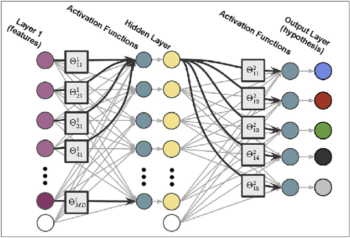
A feedforward neural network is a type of neural network that consists of an input layer, one or more hidden layers, and an output layer. The information flows only in one direction from the input layer to the output layer, hence the name “feedforward”.
Implementation of building a feedforward neural network in TensorFlow to classify the MNIST dataset, which contains images of handwritten digits:
import tensorflow as tf# Load the MNIST dataset
(x_train, y_train), (x_test, y_test) = tf.keras.datasets.mnist.load_data()x_train = x_train.reshape(x_train.shape[0], 28 * 28) / 255.0
x_test = x_test.reshape(x_test.shape[0], 28 * 28) / 255.0# One-hot encode the labels
y_train = tf.keras.utils.to_categorical(y_train, 10)
y_test = tf.keras.utils.to_categorical(y_test, 10)# Define the model architecture
model = tf.keras.models.Sequential([
tf.keras.layers.Dense(128, input_shape=(28 * 28,), activation='relu'),
tf.keras.layers.Dense(64, activation='relu'),
tf.keras.layers.Dense(10, activation='softmax')
])# Compile the model
model.compile(loss='categorical_crossentropy', optimizer='adam', metrics=['accuracy'])# Train the model
history = model.fit(x_train, y_train, batch_size=64, epochs=10, verbose=1, validation_data=(x_test, y_test))# Evaluate the model on the test data
test_loss, test_accuracy = model.evaluate(x_test, y_test, verbose=0)
print('Test loss:', test_loss)
print('Test accuracy:', test_accuracy)In this implementation, the model consists of three dense (fully-connected) layers with 128, 64, and 10 neurons, respectively. The first layer takes the 28 x 28 images as input and has 128 neurons. The second layer has 64 neurons, and the third layer has 10 neurons, which correspond to the 10 classes in the MNIST dataset. The activation function for the first two layers is the ReLU activation function, and the activation function for the final layer is the softmax activation function, which produces probability scores for each class.
The model is compiled with the categorical cross-entropy loss function and the Adam optimizer. The fit function trains the model for 10 epochs with a batch size of 64. Finally, the model is evaluated on the test data and its performance is reported.
A feedforward neural network is a type of artificial brain that is designed to take in information, process it, and give an output.
It’s kind of like a calculator, but much more powerful!
- The way it works is that you have different layers of neurons, and each layer processes the information a little bit before passing it on to the next layer. Imagine you’re trying to teach a computer to recognize different animals. The first layer of neurons might look at the color of the animal, and pass that information on to the next layer. The next layer might look at the shape of the animal, and so on.
- Each neuron in the network is connected to other neurons in the previous and next layers, and each connection has a weight that determines how important that input is to the output. Think of it like a team of superheroes working together to save the world — each one has their own special power, but they need to work together and use their powers in just the right way to be successful.
- Once all the layers have processed the information, the network gives an output — in this case, whether it thinks the animal is a dog, a cat, or something else. The network can learn from its mistakes and adjust the weights of the connections to make better predictions over time.
So, a feedforward neural network is a powerful tool that can help us recognize patterns and make predictions based on input data. It’s like having a team of superheroes working together to solve a problem!
Backpropagation
Backpropagation is the algorithm used to update the weights of a neural network during training. It works by calculating the gradient of the loss function with respect to each weight in the network, and then using that gradient to update the weight in the opposite direction of the gradient.
Implementation of how to use backpropagation to train a simple neural network in Keras:
from tensorflow.keras.models import Sequential
from tensorflow.keras.layers import Dense
from tensorflow.keras.optimizers import SGD
# define a simple neural network model
model = Sequential()
model.add(Dense(10, input_shape=(5,), activation='relu'))
model.add(Dense(1, activation='sigmoid'))# compile the model with stochastic gradient descent optimizer
sgd = SGD(lr=0.1)
model.compile(optimizer=sgd, loss='binary_crossentropy')# train the model with backpropagation
model.fit(X_train, y_train, epochs=100)In this implementation, we first define a simple neural network with two layers, and compile it with the stochastic gradient descent (SGD) optimizer and binary cross-entropy loss function. The lr parameter specifies the learning rate, which determines how quickly the weights of the network are updated.
Next, we train the model with the fit function, which uses backpropagation to update the weights of the network during each epoch of training. The epochs parameter specifies the number of times to iterate over the training data.
During each iteration, the backpropagation algorithm calculates the gradient of the loss function with respect to each weight in the network, and updates the weights in the opposite direction of the gradient. This process is repeated for each iteration until the loss function is minimized, and the network is considered to be trained.
The algorithm uses gradient descent to find the minimum error. The gradient of the error with respect to the weights and biases of the neurons is computed using the chain rule of differentiation. The gradient is then used to update the weights and biases in the direction of the minimum error.
Implementation of how backpropagation can be implemented:
import numpy as npdef sigmoid(x):
return 1/(1+np.exp(-x))def sigmoid_derivative(x):
return x * (1 - x)# Input dataset
X = np.array([ [0,0,1],
[0,1,1],
[1,0,1],
[1,1,1] ])# Output dataset
y = np.array([[0,0,1,1]]).T# Seed the random number generator
np.random.seed(1)# Initialize weights randomly with mean 0
weights0 = 2*np.random.random((3,1)) - 1for iteration in range(10000): # Forward pass
layer0 = X
layer1 = sigmoid(np.dot(layer0,weights0)) # Compute error
layer1_error = y - layer1 # Backpropagation
layer1_delta = layer1_error * sigmoid_derivative(layer1) # Update weights
weights0 += np.dot(layer0.T,layer1_delta)print("Output After Training:")
print(layer1)In this implementation, we first define a sigmoid function, which is used as the activation function for the neurons in the network, and its derivative. Then, we create a simple XOR dataset and initialize the weights randomly with a mean of 0. In each iteration of the loop, the forward pass computes the output of the network given the input and weights. The error is then computed and used to update the weights in the direction of the minimum error using backpropagation.
Backpropagation is a key algorithm in deep learning, as it allows neural networks to learn complex patterns from data. By iteratively updating the weights of the network using the gradient of the loss function, backpropagation enables the network to adjust its parameters and improve its predictions over time.
- Imagine you’re playing a game where you have to guess what animal your friend is thinking of. Your friend thinks of an animal, and gives you a hint — “it has four legs.” You guess “dog,” but your friend says it’s not a dog. You keep guessing until you finally guess “cat,” and your friend says that’s the right answer.
- In a way, training a neural network is like playing this game with the computer. The computer has to guess what the right answer is based on some hints, or data, that we give it. We show the computer lots of examples of things we want it to learn, like pictures of dogs and cats, and we tell it what each picture is.
- Backpropagation is like a way for the computer to learn from its mistakes, just like you learned from your wrong guesses when playing the game with your friend. When the computer makes a guess, we tell it if it’s right or wrong, and then it tries to adjust its guess to be better next time.
- But how does the computer know how to adjust its guess? Backpropagation is like a teacher that helps the computer figure that out. The teacher looks at the computer’s guess, and then helps it adjust the “weights” of the network — kind of like knobs that control how the computer processes the data. The teacher helps the computer change the weights so that it makes better guesses next time.
So, in short, backpropagation is like a teacher that helps the computer learn from its mistakes, by adjusting the weights of the neural network to make better guesses next time. Just like you learned from your mistakes when playing the game with your friend, backpropagation helps the computer learn and improve its guesses over time.
Activation functions
Activation functions are an important component of neural networks. They determine the output of a neuron in response to the inputs it receives from other neurons. The activation function maps the inputs to the output, and different activation functions have different properties that make them suitable for different types of neural networks and tasks.
Implementation of how to implement different activation functions in TensorFlow:
import tensorflow as tf# Sigmoid activation function
def sigmoid(x):
return 1 / (1 + tf.exp(-x))# ReLU activation function
def relu(x):
return tf.maximum(0, x)# Tanh activation function
def tanh(x):
return tf.tanh(x)# Softmax activation function
def softmax(x):
return tf.nn.softmax(x)# Example input
x = tf.constant([-2.0, -1.0, 0.0, 1.0, 2.0], dtype=tf.float32)# Apply each activation function to the input
sigmoid_output = sigmoid(x)
relu_output = relu(x)
tanh_output = tanh(x)
softmax_output = softmax(x)print('Sigmoid output:', sigmoid_output.numpy())
print('ReLU output:', relu_output.numpy())
print('Tanh output:', tanh_output.numpy())
print('Softmax output:', softmax_output.numpy())In this implementation, we have defined four different activation functions: sigmoid, ReLU, tanh, and softmax. The input x is a constant tensor with 5 values. We apply each activation function to the input and print the output. The sigmoid activation function maps the input to values between 0 and 1, which can be interpreted as probabilities. The ReLU activation function sets negative values to 0 and leaves positive values unchanged, which can improve the training speed and prevent the vanishing gradient problem. The tanh activation function maps the input to values between -1 and 1. The softmax activation function maps the input to a probability distribution over multiple classes.
An activation function is a function that helps a neural network decide how important each input is for making a prediction. It’s kind of like a filter that helps the network figure out what’s important and what’s not.
- Let’s say you’re trying to teach a computer to recognize different animals. You might have a bunch of inputs, like the color of the animal, the shape of its ears, and how big it is. An activation function looks at all of these inputs and decides which ones are most important for predicting what kind of animal it is.
- Think of it like a traffic light — it helps the neural network decide when to “turn on” and start making predictions. If the input is important, the activation function will “turn on” and let the network know to pay attention to that input. If it’s not important, the activation function will “turn off” and the network will ignore it.
- There are many different types of activation functions, each with its own strengths and weaknesses. Some are good at recognizing patterns in images, while others are better at predicting numerical values.
So, an activation function is a kind of filter that helps a neural network figure out which inputs are important for making a prediction. It’s like a traffic light that tells the network when to pay attention and when to ignore certain inputs.
Strategy for Reducing Errors
There are several strategies for reducing errors in deep learning :
- Data preprocessing and augmentation: Clean and preprocess the input data to remove outliers, normalize the features, and increase the size of the dataset with data augmentation techniques such as rotation, flipping, and scaling.
- Architecture design: Choose a suitable neural network architecture for the task, such as a convolutional neural network for image classification or a recurrent neural network for time series prediction.
- Hyperparameter tuning: Experiment with different hyperparameters such as learning rate, batch size, and number of hidden units to find the best values that minimize the error.
- Regularization: Add regularization terms to the loss function, such as L2 regularization or dropout, to prevent overfitting and reduce the error.
- Early stopping: Monitor the performance on a validation set and stop training when the error starts to increase, to avoid overfitting.
Implementation of how to implement early stopping in TensorFlow:
import tensorflow as tf# Load the MNIST dataset
(x_train, y_train), (x_test, y_test) = tf.keras.datasets.mnist.load_data()
x_train = x_train / 255.0
x_test = x_test / 255.0# Define the model
model = tf.keras.models.Sequential([
tf.keras.layers.Flatten(input_shape=(28, 28)),
tf.keras.layers.Dense(128, activation='relu'),
tf.keras.layers.Dense(10, activation='softmax')
])# Compile the model
model.compile(optimizer='adam', loss='sparse_categorical_crossentropy', metrics=['accuracy'])# Define the early stopping callback
early_stopping = tf.keras.callbacks.EarlyStopping(monitor='val_loss', patience=3)# Train the model
history = model.fit(x_train, y_train, validation_split=0.1, epochs=100, callbacks=[early_stopping])In this implementation, we load the MNIST dataset and define a simple feedforward neural network with two dense layers. We compile the model with the Adam optimizer and the sparse categorical crossentropy loss. We also define an early stopping callback that monitors the validation loss and stops training after 3 epochs without improvement. Finally, we fit the model to the training data and store the training history in the history variable. The model will automatically stop training when the validation loss starts to increase, which is a sign of overfitting.
Deep learning is like teaching the computer to learn, just like how you learn new things every day. But sometimes, the computer can get a little too excited and learn too much, which can make it forget some of the important things it’s already learned.
- To help the computer learn better, we use something called “early stopping.” It’s like when we play a game and we have to stop after a certain amount of time, even if we haven’t finished the game yet. We stop playing so that we can remember what we already learned, and then we can come back and finish the game later.
- Early stopping works the same way for computers. When we’re teaching the computer to learn, we stop the computer from learning after a certain amount of time, even if it hasn’t learned everything yet. This helps the computer remember what it has already learned, and then it can come back and learn more later.
So early stopping is like taking a break when we’re learning, so we can remember what we’ve learned and then keep learning more later.
Convolutional Neural Network
A Convolutional Neural Network (ConvNet/CNN) is a type of neural network that is commonly used for image classification and computer vision tasks.
The key idea behind ConvNets is to use convolutional layers to extract local features from the input image and pooling layers to reduce the spatial dimensions.
Implementation of a simple ConvNet in TensorFlow:
import tensorflow as tf# Load the CIFAR-10 dataset
(x_train, y_train), (x_test, y_test) = tf.keras.datasets.cifar10.load_data()
x_train = x_train / 255.0
x_test = x_test / 255.0# Define the model
model = tf.keras.models.Sequential([
tf.keras.layers.Conv2D(32, (3, 3), activation='relu', input_shape=(32, 32, 3)),
tf.keras.layers.MaxPooling2D((2, 2)),
tf.keras.layers.Conv2D(64, (3, 3), activation='relu'),
tf.keras.layers.MaxPooling2D((2, 2)),
tf.keras.layers.Flatten(),
tf.keras.layers.Dense(64, activation='relu'),
tf.keras.layers.Dense(10, activation='softmax')
])# Compile the model
model.compile(optimizer='adam', loss='sparse_categorical_crossentropy', metrics=['accuracy'])# Train the model
history = model.fit(x_train, y_train, validation_split=0.1, epochs=10)In this implementation, we load the CIFAR-10 dataset and define a ConvNet with two convolutional layers, each followed by a max pooling layer. The convolutional layers use a ReLU activation function and a 3x3 kernel size, and the max pooling layers reduce the spatial dimensions by a factor of 2. We also add two dense layers at the end of the network to produce the final classification. We compile the model with the Adam optimizer and the sparse categorical crossentropy loss, and train the model for 10 epochs with a validation split of 10%. The model will learn to extract local features from the input images and use them to classify the images into one of 10 classes.
Convolutional Neural Networks are like a special kind of teacher that helps the computer understand pictures and videos. It’s like how your teacher helps you learn new things in school, but for pictures and videos.
- So when we want the computer to learn how to recognize a picture, we show it lots of different pictures and tell it what’s in each picture. The computer then uses the Convolutional Neural Network to look at each picture really closely, kind of like how you look at a picture with a magnifying glass.
- The Convolutional Neural Network helps the computer find special patterns in the picture that help it recognize what’s in the picture. It’s like when you look at a picture and notice that there are a lot of trees in it, or that there’s a big blue sky.
- Once the computer has looked at lots of pictures and found all the special patterns, it can use that information to recognize new pictures it’s never seen before. It’s like when you learn how to count to 10, and then you can count anything you see, even if you’ve never seen it before.
So that’s what Convolutional Neural Networks are! They’re a special kind of teacher that helps computers understand pictures and videos, and then recognize new ones.
The basic building blocks of a ConvNet are the convolutional layer, pooling layer, activation function, and dense layer.
A ConvNet architecture typically consists of multiple convolutional layers followed by pooling layers, activation functions, and dense layers. The convolutional layers extract local features from the input image, and the pooling layers reduce the spatial dimensions to allow for translation invariance. The activation functions introduce non-linearities into the model, and the dense layers make predictions based on the extracted features.
Implement a simple ConvNet in TensorFlow:
import tensorflow as tf# Load the MNIST dataset
(x_train, y_train), (x_test, y_test) = tf.keras.datasets.mnist.load_data()
x_train = x_train / 255.0
x_test = x_test / 255.0
x_train = x_train[..., tf.newaxis]
x_test = x_test[..., tf.newaxis]# Define the model
model = tf.keras.models.Sequential([
tf.keras.layers.Conv2D(32, (3, 3), activation='relu', input_shape=(28, 28, 1)),
tf.keras.layers.MaxPooling2D((2, 2)),
tf.keras.layers.Flatten(),
tf.keras.layers.Dense(64, activation='relu'),
tf.keras.layers.Dense(10, activation='softmax')
])# Compile the model
model.compile(optimizer='adam', loss='sparse_categorical_crossentropy', metrics=['accuracy'])# Train the model
history = model.fit(x_train, y_train, validation_split=0.1, epochs=10)In this implementation, we load the MNIST dataset and define a ConvNet with one convolutional layer, one max pooling layer, and two dense layers. The convolutional layer uses a 3x3 kernel size, a ReLU activation function, and an input shape of 28x28x1. The max pooling layer reduces the spatial dimensions by a factor of 2. The dense layers use a ReLU activation function for the hidden layer and a softmax activation function for the output layer. We compile the model with the Adam optimizer, the sparse categorical crossentropy loss, and accuracy as the metric. Finally, we train the model for 10 epochs with a validation split of 10%.
CNN architectures are like different blueprints for building a really cool treehouse. They tell us how to build the treehouse, what materials to use, and what kind of cool features to add.
- In the same way, CNN architectures tell us how to build the Convolutional Neural Network, what kind of layers to use, and how to put them together. Different architectures can have different layers and different ways of putting them together, kind of like how different treehouses can have different rooms and different ways of connecting them.
- Some CNN architectures are really good at recognizing certain kinds of pictures, like pictures of animals or cars. Other architectures might be better at recognizing different things, like faces or buildings.
- Just like how different treehouses can be better for different things, like playing or reading or sleeping, different CNN architectures can be better for different kinds of pictures and videos. So people who use CNNs choose different architectures based on what they want the computer to be able to do.
That’s what CNN architectures are! They’re like different blueprints for building a really cool treehouse, but instead of building a treehouse, we’re building a computer program that can understand pictures and videos.
Recurrent Neural Network (RNN)
A Recurrent Neural Network (RNN) is a type of neural network designed to process sequences of data, such as sequences of words in natural language processing or sequences of frames in video analysis. An RNN contains a hidden state that can be updated at each time step based on the input and previous hidden state, allowing it to capture dependencies between elements in the sequence.
Implementation of building an RNN in TensorFlow:
import tensorflow as tf
import numpy as np
# Define the model architecture
model = tf.keras.models.Sequential([
tf.keras.layers.Embedding(vocab_size, 128, input_length=max_len),
tf.keras.layers.LSTM(64),
tf.keras.layers.Dense(1, activation='sigmoid')
])# Compile the model
model.compile(optimizer='adam', loss='binary_crossentropy', metrics=['accuracy'])# Generate dummy data
num_samples = 1000
max_len = 10
vocab_size = 100x = np.random.randint(0, vocab_size, (num_samples, max_len))
y = np.random.randint(0, 2, num_samples)# Train the model
history = model.fit(x, y, epochs=10)In this implementation, we define a simple RNN with an embedding layer, an LSTM (Long Short-Term Memory) layer, and a dense layer with a sigmoid activation function. The embedding layer maps the input sequences of integers to a lower-dimensional space, and the LSTM layer captures dependencies between elements in the sequences. The dense layer outputs a binary classification result. We compile the model with the Adam optimizer, the binary crossentropy loss, and accuracy as the metric. Finally, we generate some dummy data and train the model for 10 epochs.
Recurrent Neural Networks are like a special kind of teacher that helps the computer understand how to use words and sentences. It’s like when your teacher helps you learn how to write a story, but for a computer.
- So when we want the computer to learn how to write a story, we show it lots of different stories and tell it what happens in each one. The computer then uses the Recurrent Neural Network to read each story really closely, kind of like how you read a story with your eyes.
- The Recurrent Neural Network helps the computer remember what happened in the story, and also helps it understand how the story is put together. It’s like when you read a story and notice how the beginning, middle, and end are all connected.
- Once the computer has read lots of stories and understands how they work, it can use that information to write new stories that it’s never seen before. It’s like when you learn how to write a story, and then you can write any story you want, even if you’ve never seen it before.
So that’s what Recurrent Neural Networks are! They’re a special kind of teacher that helps computers understand words and sentences, and then use that understanding to write new things.
Custom Loss functions
Custom loss functions are an essential part of deep learning, allowing you to fine-tune the performance of your model for specific tasks. A custom loss function can be defined as a way to calculate the difference between the actual output and the desired output, which is then used to update the weights and biases of the model during training. In other words, the loss function is used to optimize the model, so it can better predict the target outputs.
Implementation in Python using TensorFlow 2.x:
import tensorflow as tfdef custom_loss(y_true, y_pred):
# Define the custom loss function
loss = tf.reduce_mean(tf.square(y_true - y_pred))
return loss# Compile the model using the custom loss function
model.compile(optimizer='adam', loss=custom_loss)In this implementation, the custom loss function is defined as the mean squared error between the actual outputs y_true and the predicted outputs y_pred. The tf.reduce_mean function is used to calculate the average of the squared error across all samples in the batch.
Once the custom loss function is defined, you can compile the model using it by passing it as the loss argument when compiling the model. This will ensure that the model uses the custom loss function during the training process.
Custom Loss Functions are like a special set of rules that help the computer know when it’s doing a good job and when it’s not. It’s like when you play a game and you know you’re doing a good job because you get points, or you know you’re not doing a good job because you lose a life.
- When we use a Custom Loss Function, we’re telling the computer exactly what it needs to do to be successful. For example, if we want the computer to recognize only pictures of dogs, we would use a Custom Loss Function that rewards the computer for recognizing dogs and punishes it for recognizing anything else. It’s like giving the computer a special set of rules that it has to follow in order to win the game.
- Once the computer knows the rules, it can use them to get better at recognizing pictures of dogs. It’s like when you play a game and you start getting better because you understand the rules.
So that’s what Custom Loss Functions are! They’re a special set of rules that we give to the computer to help it know when it’s doing a good job and when it’s not. By using these rules, we can teach the computer to do really specific things, like recognizing only pictures of dogs.
NLP and Word Embeddings
Natural Language Processing is a subfield of computer science and artificial intelligence that focuses on enabling computers to understand, interpret, and generate human language. It involves many techniques, such as text pre-processing, feature extraction, and machine learning models.
One important technique in NLP is word embeddings.
Word embeddings are a way of representing words as vectors (i.e., arrays of numbers). These vectors capture the meaning of words in a way that allows them to be used as input to machine learning models.
There are many different algorithms for generating word embeddings, but a popular one is Word2Vec.
Implementation of how to use Word2Vec to generate word embeddings for a set of sentences:
import gensim
from gensim.models import Word2Vec
# create a list of sentences
sentences = [["the", "quick", "brown", "fox", "jumps", "over", "the", "lazy", "dog"],
["i", "love", "machine", "learning"],
["natural", "language", "processing", "is", "fun"]]# create a Word2Vec model and train it on the sentences
model = Word2Vec(sentences, min_count=1)# get the embedding for a word
vector = model.wv['machine']
print(vector)In this code, we first create a list of sentences. We then create a Word2Vec model and train it on the sentences. Finally, we get the word embedding for the word “machine” and print it out. This code will output a 100-dimensional vector representing the word “machine”. This vector captures the meaning of the word in a way that can be used as input to a machine learning model.
Word embeddings are a powerful technique in NLP because they allow us to use machine learning models to process natural language text. We can use them to do things like text classification, sentiment analysis, and machine translation.
Imagine you and your friends have a secret language that only you can understand. You might have a special word for “pizza”, and another special word for “ice cream”. Even if someone else heard you say those words, they wouldn’t know what you were talking about, because they don’t know the secret code.
- Word embeddings are kind of like that secret language. They help computers understand what words mean by giving each word a special code. This code is like a special number that the computer can use to represent the word.
- For example, imagine we have a computer program that knows about cats and dogs. We could give it a special code for the word “cat”, and a different special code for the word “dog”. Then, when the program sees the word “cat” or “dog” in a sentence, it can use the special code to figure out what the word means.
So, in summary, word embeddings are special codes that help computers understand what words mean. These codes make it easier for computers to work with words and sentences in natural language, just like a secret code can make it easier for you to talk with your friends without anyone else understanding what you’re saying.
Callbacks
Callbacks are functions that you can specify to be called at certain points during the training of a neural network. They allow you to perform actions such as saving the best model, stopping training early, or modifying the learning rate during training.
Implementation of how to use a callback in Keras to save the best model during training:
from tensorflow.keras.models import Sequential
from tensorflow.keras.layers import Dense
from tensorflow.keras.callbacks import ModelCheckpoint
# define a simple neural network model
model = Sequential()
model.add(Dense(10, input_shape=(5,), activation='relu'))
model.add(Dense(1, activation='sigmoid'))# compile the model
model.compile(optimizer='adam', loss='binary_crossentropy')# define a checkpoint callback to save the best model during training
checkpoint = ModelCheckpoint('best_model.h5', monitor='val_loss', save_best_only=True)# train the model with the callback
model.fit(X_train, y_train, validation_data=(X_test, y_test), epochs=100, callbacks=[checkpoint])In this implementation, we first define a simple neural network model with two layers. We then compile the model with an optimizer and a loss function.
Next, we define a checkpoint callback using the ModelCheckpoint function. This callback will save the weights of the best model based on the validation loss. The monitor parameter specifies the quantity to monitor, and the save_best_only parameter specifies whether to save only the best model or every model.
Finally, we train the model with the callback by passing the callbacks parameter to the fit function.
Callbacks are a powerful tool in deep learning because they allow you to customize the training process of your neural network. With callbacks, you can perform actions such as saving the best model, early stopping, and modifying the learning rate during training, which can help improve the performance of your model.
Callbacks are kind of like a special helper that can watch what’s happening when you’re doing something, and then tell you when it’s time to do something special. Imagine you’re playing with your toys, and your mom tells you that it’s time to go to bed soon. She might set a timer or an alarm on her phone to remind you when it’s time to stop playing and get ready for bed.
- Callbacks work a bit like that alarm on your mom’s phone. When you’re training a computer to learn something, like recognizing pictures of dogs, the callback can watch what’s happening and remind the computer to do something special at certain times. For example, it could remind the computer to save the best model it’s learned so far, or to stop training early if it’s not learning very well.
So, in short, callbacks are like a special helper that watches what’s happening when you’re training a computer, and reminds the computer to do something special at certain times. Just like an alarm can help remind you when it’s time to do something special, callbacks can help a computer learn better by reminding it to do something special at the right time.
Implementation on how to use a callback in Keras to save the model’s weights after every epoch:
from keras.callbacks import ModelCheckpoint# define a callback to save the weights after every epoch
checkpoint = ModelCheckpoint(filepath='weights.{epoch:02d}.hdf5', save_best_only=False)# fit the model using the callback
model.fit(x_train, y_train, epochs=100, batch_size=32, callbacks=[checkpoint])In this implementation, ModelCheckpoint is a built-in Keras callback that saves the model's weights after every epoch. The filepath argument specifies the file name pattern to use when saving the weights, and the save_best_only argument determines whether to save only the best weights (based on the validation loss) or to save the weights after every epoch.
You can also define your own custom callbacks by creating a class that implements the on_epoch_end method and passing an instance of the class to the fit method as a callback. For example, here is a custom callback that stops the training process if the validation loss does not improve for 10 consecutive epochs:
from keras.callbacks import Callbackclass EarlyStoppingByLossVal(Callback):
def __init__(self, monitor='val_loss', value=0.00001, verbose=0):
super(Callback, self).__init__()
self.monitor = monitor
self.value = value
self.verbose = verbose def on_epoch_end(self, epoch, logs={}):
current = logs.get(self.monitor)
if current is None:
warnings.warn("Early stopping requires %s available!" % self.monitor, RuntimeWarning)
if current < self.value:
if self.verbose > 0:
print("Epoch %05d: early stopping THR" % epoch)
self.model.stop_training = True# define a custom callback to stop the training if the validation loss does not improve for 10 epochs
early_stopping = EarlyStoppingByLossVal(monitor='val_loss', value=0.00001, verbose=1)# fit the model using the custom callback
model.fit(x_train, y_train, epochs=100, batch_size=32, callbacks=[early_stopping])In this implementation, the EarlyStoppingByLossVal class extends the Callback class and implements the on_epoch_end method. The on_epoch_end method is called after each epoch, and it checks the value of the val_loss log to see if it is below a specified value. If it is, the method sets the stop_training attribute of the model to True, which stops the training process.
Gradient Descent
Gradient Descent is an optimization algorithm used in deep learning to update the model parameters so as to minimize the loss function. The idea behind gradient descent is simple: starting with some initial values for the model parameters, we iteratively update the parameters in the direction of the negative gradient of the loss function with respect to the parameters, until the minimum is reached.
Implementation in Python using Keras:
import tensorflow as tf
from tensorflow import keras
# Define the model
model = keras.Sequential([
keras.layers.Dense(64, activation='relu', input_shape=(32,)),
keras.layers.Dense(64, activation='relu'),
keras.layers.Dense(10, activation='softmax')
])# Compile the model with loss function and optimizer
model.compile(optimizer=tf.optimizers.SGD(learning_rate=0.01),
loss='categorical_crossentropy',
metrics=['accuracy'])# Train the model on data
history = model.fit(train_data, train_labels, epochs=10)In this implementation, we define a simple multi-layer feedforward neural network using the Sequential class from Keras. We then compile the model by specifying the optimizer, loss function, and metrics to use during training. We use the Stochastic Gradient Descent (SGD) optimizer, with a learning rate of 0.01. Finally, we train the model on the train_data and train_labels using the fit method, and run the training for 10 epochs.
Note that the learning rate determines the size of the step taken in the direction of the negative gradient during each iteration of the optimization. A smaller learning rate means that the optimization will converge more slowly but with a better chance of finding the true minimum, whereas a larger learning rate will converge faster but with a higher risk of overshooting the minimum.
Imagine you’re climbing a mountain. You start at the bottom and want to get to the top. But you can’t see the top because there are clouds covering it. So, you start by taking a step in any direction. You look around and see what the ground looks like around you. If it looks like you’re getting closer to the top, you take another step in the same direction. If you’re getting farther away, you take a step in the opposite direction. You keep doing this until you reach the top of the mountain.
- This is kind of like what gradient descent is doing when we’re training a machine learning model. The goal is to find the best values of some parameters that will allow the model to make good predictions. We start by randomly guessing some values for the parameters. Then, we look at the predictions the model makes with those values and see how well they match the real answers.
- The gradient descent algorithm looks at how much the predictions need to be improved and in which direction the parameters need to be adjusted to improve them. It then adjusts the parameters a little bit in that direction and checks how the predictions change. If the predictions are getting better, it continues to adjust the parameters in the same direction. If the predictions are getting worse, it adjusts the parameters in the opposite direction.
- Just like climbing a mountain, the algorithm repeats this process over and over again, taking small steps in the direction that will lead to better predictions until it can’t make the predictions any better.
So, in short, gradient descent is like climbing a mountain to find the best way to make good predictions with a machine learning model. You start at a random place, take small steps in the direction that will make the predictions better, and keep doing this until you find the best values of the parameters that will allow the model to make the best predictions.
Batch Normalization
Batch Normalization is a technique used in deep learning to normalize the activations of a network layer across the mini-batch. The idea behind batch normalization is to adjust the values of the activations so that they have zero mean and unit variance, making the network more stable and reducing the risk of vanishing gradients.
Implementation in Python using Keras:
import tensorflow as tf
from tensorflow import keras
# Define the model
model = keras.Sequential([
keras.layers.Dense(64, activation='relu', input_shape=(32,)),
keras.layers.BatchNormalization(),
keras.layers.Dense(64, activation='relu'),
keras.layers.BatchNormalization(),
keras.layers.Dense(10, activation='softmax')
])# Compile the model
model.compile(optimizer=tf.optimizers.SGD(learning_rate=0.01),
loss='categorical_crossentropy',
metrics=['accuracy'])# Train the model on data
history = model.fit(train_data, train_labels, epochs=10)In this implementation, we define a simple multi-layer feedforward neural network using the Sequential class from Keras. We insert a BatchNormalization layer after each fully connected layer, which normalizes the activations of that layer. We then compile the model and train it on the train_data and train_labels as before.
Batch normalization is like having a team of kids working on a big puzzle together. Each kid has their own part of the puzzle to work on, and they are all trying to put their pieces together to complete the puzzle.
- But sometimes, one kid may be working on a part of the puzzle that is too hard for them, and they are slowing down the whole team. This is kind of like what can happen in a neural network when one neuron is getting too much or too little data compared to the other neurons. This can slow down the whole network and make it harder for it to learn.
- So, what batch normalization does is make sure that all the neurons in the network are getting a fair amount of data to work with. It’s like if the kids working on the puzzle decided to divide the puzzle pieces equally between each other, so that no one kid had too many or too few pieces to work with. This would help the whole team work more efficiently and complete the puzzle faster.
- Similarly, batch normalization helps each neuron in the network get a fair amount of data to work with by adjusting the data so that the mean and standard deviation of each batch of data is the same. This makes it easier for the network to learn and make accurate predictions.
So, in short, batch normalization is like making sure all the kids working on a puzzle get an equal amount of puzzle pieces to work with, so that they can work efficiently and complete the puzzle faster. In the same way, batch normalization helps each neuron in a neural network get a fair amount of data to work with, so that the network can learn more efficiently and make accurate predictions.
Popular optimization algorithms
Optimization algorithms are used to update the weights of a neural network during training.
There are several popular optimization algorithms used in deep learning, each with their own strengths and weaknesses. Here are explanations and code examples for three of the most popular optimization algorithms: Stochastic Gradient Descent (SGD), Adam, and RMSprop.
- Stochastic Gradient Descent (SGD):
SGD is the most basic optimization algorithm used in deep learning. It works by updating the weights of the neural network in the direction of the negative gradient of the loss function with respect to the weights. This means that it will adjust the weights to make the loss smaller with each update.
Here’s an implementation of SGD in Python using the Keras library:
from keras.optimizers import SGDsgd = SGD(lr=0.01, momentum=0.9)
model.compile(optimizer=sgd, loss='categorical_crossentropy', metrics=['accuracy'])In this code, we are creating an instance of the SGD optimizer and setting the learning rate (lr) and momentum hyperparameters. We then compile the model with the optimizer, the loss function, and the metrics we want to track during training.
- Adam:
Adam is an adaptive optimization algorithm that combines the benefits of both SGD and RMSprop. It uses moving averages of the gradient and the second moment of the gradient to update the weights. This means that it can adapt to the geometry of the loss function and perform better on non-convex optimization problems.
Here’s an implementation of Adam in Python using Keras:
from keras.optimizers import Adamadam = Adam(lr=0.001, beta_1=0.9, beta_2=0.999)
model.compile(optimizer=adam, loss='categorical_crossentropy', metrics=['accuracy'])In this code, we are creating an instance of the Adam optimizer and setting the learning rate (lr), beta_1, and beta_2 hyperparameters. We then compile the model with the optimizer, the loss function, and the metrics we want to track during training.
- RMSprop:
RMSprop is an adaptive optimization algorithm that uses a moving average of the squared gradient to update the weights. It has been shown to perform well on deep neural networks and can adapt to the geometry of the loss function.
Here’s an implementation of RMSprop in Python using Keras:
from keras.optimizers import RMSproprmsprop = RMSprop(lr=0.001, rho=0.9)
model.compile(optimizer=rmsprop, loss='categorical_crossentropy', metrics=['accuracy'])In this code, we are creating an instance of the RMSprop optimizer and setting the learning rate (lr) and rho hyperparameters. We then compile the model with the optimizer, the loss function, and the metrics we want to track during training.
- Stochastic Gradient Descent (SGD): SGD is like a coach that tells the computer which way to run in order to get better at answering questions. The coach watches the computer try to answer a question, and then tells it how to adjust its thinking in order to get closer to the right answer. It does this over and over again, getting a little better each time, until it gets really good at answering questions.
- Adam: Adam is like a magic genie that helps the computer learn faster. It looks at how the computer is trying to solve the problem, and figures out the best way to adjust its thinking in order to get better answers. It’s really good at finding the right adjustments to make, so the computer can learn much faster than it would with just SGD.
- RMSprop: RMSprop is like a scientist that studies the computer’s progress and figures out the best way to make it better. It watches the computer try to answer questions, and figures out which adjustments are making the biggest difference. Then it focuses on those adjustments, and helps the computer make even more progress.
Shallow Neural network
A shallow neural network is a neural network that has only one hidden layer, or a small number of hidden layers. Shallow neural networks are a type of feedforward neural network and are often used as a simple building block for more complex neural networks.
Here’s a code implementation in Python using Keras:
import tensorflow as tf
from tensorflow import keras
# Define the model
model = keras.Sequential([
keras.layers.Dense(64, activation='relu', input_shape=(32,)),
keras.layers.Dense(10, activation='softmax')
])# Compile the model
model.compile(optimizer=tf.optimizers.SGD(learning_rate=0.01),
loss='categorical_crossentropy',
metrics=['accuracy'])# Train the model on data
history = model.fit(train_data, train_labels, epochs=10)In this implementation, we define a simple shallow neural network using the Sequential class from Keras. The network consists of only two fully connected (dense) layers, with a ReLU activation for the first layer and a softmax activation for the final output layer. We compile the model using the SGD optimizer, with a learning rate of 0.01, and train it on the train_data and train_labels as before.
A shallow neural network is like a group of little detectives working together to solve a mystery. Each detective (or “neuron”) takes a look at a small piece of the evidence, and tries to figure out what it means. Then, they all get together to share what they found, and try to make sense of the big picture.
To create a shallow neural network, we first gather a bunch of data and labels, like pictures of animals and their names. Then, we train the network by showing it the pictures and asking it to guess the name of the animal in the picture. If it guesses wrong, we give it a little nudge in the right direction so that it can do better next time.
Residual Networks
Residual networks, also known as ResNets, are a type of deep neural network that were introduced to address the issue of vanishing gradients in deep neural networks. In a residual network, instead of trying to learn an end-to-end mapping from inputs to outputs, the network learns to learn a residual mapping, that is, the difference between the desired mapping and a simple baseline mapping.
Implementation in Python using Keras:
import tensorflow as tf
from tensorflow import keras
def residual_block(inputs, filters, stride=1):
x = keras.layers.Conv2D(filters, 3, strides=stride, padding='same')(inputs)
x = keras.layers.BatchNormalization()(x)
x = keras.layers.ReLU()(x)
x = keras.layers.Conv2D(filters, 3, strides=1, padding='same')(x)
x = keras.layers.BatchNormalization()(x)
shortcut = keras.layers.Conv2D(filters, 1, strides=stride, padding='same')(inputs)
x = keras.layers.add([x, shortcut])
x = keras.layers.ReLU()(x)
return x# Define the model
inputs = keras.Input(shape=(224,224,3))
x = keras.layers.Conv2D(64, 7, strides=2, padding='same')(inputs)
x = keras.layers.BatchNormalization()(x)
x = keras.layers.ReLU()(x)
x = keras.layers.MaxPooling2D(3, strides=2, padding='same')(x)
for i in range(3):
x = residual_block(x, 64)
x = keras.layers.GlobalAveragePooling2D()(x)
x = keras.layers.Dense(10, activation='softmax')(x)
model = keras.Model(inputs, x)# Compile the model
model.compile(optimizer=tf.optimizers.SGD(learning_rate=0.01),
loss='categorical_crossentropy',
metrics=['accuracy'])# Train the model on data
history = model.fit(train_data, train_labels, epochs=10)In this implementation, we define a simple residual network using the Model class from Keras. The network consists of several residual blocks, each of which contains two convolutional layers and a shortcut connection that adds the input to the output of the two convolutional layers. We use batch normalization after each convolutional layer and ReLU activation after each residual block. Finally, we use a global average pooling layer to reduce the spatial dimensions of the feature maps and a dense layer to produce the final output.
A Residual Network (or “ResNet” for short) is like a team of superheroes working together to save the day. Each superhero (or “layer”) has its own special power, but they all work together to overcome any obstacle in their way.
To create a ResNet, we first gather a bunch of data and labels, like pictures of animals and their names. Then, we build a network of layers, each of which can transform the data in a different way. But instead of just passing the data through each layer one by one, like a normal network, we add a shortcut that lets the data bypass some of the layers and go straight to the next layer. This shortcut is like a secret passage that the superheroes can use to get around any obstacles in their way.
Batch Normalization and Dropout
Batch Normalization and Dropout are two popular regularization techniques in deep learning that are used to improve the performance and stability of neural networks.
Batch Normalization is a technique that normalizes the activations of each layer in a neural network across mini-batch samples. This helps to reduce the internal covariate shift and stabilize the training process. Batch normalization is typically applied after each linear operation (such as a fully connected layer or a convolutional layer) and before the activation function.
Implement Batch Normalization in Python using Keras:
import tensorflow as tf
from tensorflow import keras
# Define the model
inputs = keras.Input(shape=(224,224,3))
x = keras.layers.Conv2D(32, 3, activation='relu')(inputs)
x = keras.layers.BatchNormalization()(x)
x = keras.layers.Conv2D(64, 3, activation='relu')(x)
x = keras.layers.BatchNormalization()(x)
x = keras.layers.MaxPooling2D(2)(x)
x = keras.layers.Flatten()(x)
x = keras.layers.Dense(64, activation='relu')(x)
x = keras.layers.BatchNormalization()(x)
x = keras.layers.Dense(10, activation='softmax')(x)
model = keras.Model(inputs, x)# Compile the model
model.compile(optimizer=tf.optimizers.SGD(learning_rate=0.01),
loss='categorical_crossentropy',
metrics=['accuracy'])# Train the model on data
history = model.fit(train_data, train_labels, epochs=10)Dropout is another regularization technique that helps to reduce overfitting by randomly dropping out (i.e., setting to zero) some neurons in the network during training. Dropout is typically applied after a fully connected layer and before the activation function.
Implement Dropout in Python using Keras:
import tensorflow as tf
from tensorflow import keras
# Define the model
inputs = keras.Input(shape=(224,224,3))
x = keras.layers.Conv2D(32, 3, activation='relu')(inputs)
x = keras.layers.Conv2D(64, 3, activation='relu')(x)
x = keras.layers.MaxPooling2D(2)(x)
x = keras.layers.Flatten()(x)
x = keras.layers.Dense(64, activation='relu')(x)
x = keras.layers.Dropout(0.5)(x)
x = keras.layers.Dense(10, activation='softmax')(x)
model = keras.Model(inputs, x)# Compile the model
model.compile(optimizer=tf.optimizers.SGD(learning_rate=0.01),
loss='categorical_crossentropy',
metrics=['accuracy'])# Train the model on data
history = model.fit(train_data, train_labels, epochs=10)In this implementation, the Dropout layer is added after the dense layer with 64 units and before the final dense layer with 10 units. The dropout rate is set to 0.5, meaning that during each training iteration, half of the neurons in the dense layer will be set to zero.
LSTM (Long Short-Term Memory)
LSTM (Long Short-Term Memory) is a type of Recurrent Neural Network (RNN) that is designed to handle the problem of vanishing gradients in traditional RNNs.
LSTMs are widely used in many sequential data tasks, such as language modeling, speech recognition, and machine translation.
Implement an LSTM in Python using Keras:
import tensorflow as tf
from tensorflow import keras
# Define the model
model = keras.Sequential([
keras.layers.Embedding(vocab_size, 128),
keras.layers.LSTM(64, return_sequences=True),
keras.layers.LSTM(32),
keras.layers.Dense(10, activation='softmax')
])# Compile the model
model.compile(optimizer=tf.optimizers.Adam(learning_rate=0.01),
loss='categorical_crossentropy',
metrics=['accuracy'])# Train the model on data
history = model.fit(train_data, train_labels, epochs=10)In this implementation, we first use an Embedding layer to convert the input sequences into dense vectors with a size of 128. Then, two LSTM layers are used, with the first LSTM layer having 64 units and returning the sequence, and the second LSTM layer having 32 units and not returning the sequence. Finally, a dense layer with 10 units and a softmax activation is used to produce the output predictions. The model is then compiled with the Adam optimizer and trained on the training data.
LSTM stands for Long Short-Term Memory, and it is a type of neural network used in deep learning. Just like how our brains remember things, an LSTM network is designed to remember information over a long period of time.
- Imagine that you are reading a book, and you need to remember what happened in the beginning of the story to understand what is happening now. An LSTM network works in a similar way — it remembers what happened earlier in the input and uses that information to better understand what is happening now.
- Let me try to give you an example using a story. Let’s say that you are reading a story about a cat named Whiskers. In the beginning of the story, Whiskers is lost in the woods and is scared. As you keep reading, Whiskers meets a friendly dog named Max, who helps Whiskers find his way back home.
An LSTM network would be able to remember that Whiskers was scared and lost at the beginning of the story, and would use that information to better understand why Whiskers was so happy when he found Max.
Tensorflow
TensorFlow is a popular open-source machine learning framework developed by Google. It provides a comprehensive and flexible platform for building, training, and deploying machine learning models.
In TensorFlow, computations are expressed as a computational graph, and TensorFlow takes care of the low-level details such as memory management and optimized execution of the graph on various hardware platforms, such as CPUs and GPUs.
Implementation of how to implement a simple TensorFlow computation in Python:
import tensorflow as tf# Define two constant tensors
a = tf.constant(3.0)
b = tf.constant(4.0)# Define the computation
c = a + b# Create a TensorFlow session and run the computation
with tf.Session() as sess:
result = sess.run(c)
print("Result:", result)In this implementation, two constant tensors a and b are defined with values 3.0 and 4.0, respectively. Then, a simple computation c = a + b is defined. Finally, a TensorFlow session is created, and the computation is run using the run method of the session. The result of the computation is then printed.
TensorFlow also provides a high-level API called tf.keras for building and training machine learning models.
Implementation on how to use tf.keras to build a simple feedforward neural network:
import tensorflow as tf# Define the model
model = tf.keras.Sequential([
tf.keras.layers.Flatten(input_shape=(28, 28)),
tf.keras.layers.Dense(128, activation='relu'),
tf.keras.layers.Dense(10, activation='softmax')
])# Compile the model
model.compile(optimizer=tf.optimizers.Adam(0.001),
loss='categorical_crossentropy',
metrics=['accuracy'])# Train the model on data
history = model.fit(train_data, train_labels, epochs=10)In this implementation, a sequential model is defined using the Sequential class from tf.keras. The model consists of a flatten layer, a dense layer with 128 units and a relu activation, and a dense output layer with 10 units and a softmax activation. The model is then compiled with the Adam optimizer and a categorical cross-entropy loss function, and trained on the training data for 10 epochs.
TensorFlow is a tool that helps computers learn things, like recognizing images of animals or understanding what people say. Just like how we need to learn things step by step, TensorFlow also breaks down learning into steps.
Implementation of how you can use TensorFlow to teach a computer how to recognize images of cats and dogs:
- First, you need to give TensorFlow some pictures of cats and dogs so it can learn what they look like. This is called the training data.
- Next, you tell TensorFlow what you want it to learn, which in this case is how to recognize if an image is a cat or a dog.
- TensorFlow then takes the training data and starts looking for patterns that help it tell cats and dogs apart. It keeps adjusting itself until it can tell the difference between a cat and a dog pretty well.
- Finally, you give TensorFlow some new pictures of cats and dogs that it hasn’t seen before, and it tries to figure out if each picture is a cat or a dog. This is called the testing phase.
Implementation of how you can use TensorFlow in Python to train a simple model to recognize handwritten digits:
import tensorflow as tf# load the MNIST dataset
mnist = tf.keras.datasets.mnist
(X_train, y_train), (X_test, y_test) = mnist.load_data()# normalize the pixel values
X_train, X_test = X_train / 255.0, X_test / 255.0# create the model
model = tf.keras.models.Sequential([
tf.keras.layers.Flatten(input_shape=(28, 28)),
tf.keras.layers.Dense(128, activation='relu'),
tf.keras.layers.Dropout(0.2),
tf.keras.layers.Dense(10)
])# compile the model
model.compile(optimizer='adam',
loss=tf.keras.losses.SparseCategoricalCrossentropy(from_logits=True),
metrics=['accuracy'])# train the model
model.fit(X_train, y_train, epochs=5)# evaluate the model
model.evaluate(X_test, y_test)In this code, we are using TensorFlow to train a model to recognize handwritten digits from the MNIST dataset. We first load the dataset and normalize the pixel values. We then create a model with a flatten layer, two dense layers, and a dropout layer. We compile the model with the Adam optimizer, sparse categorical cross-entropy loss, and accuracy metric. We then train the model for 5 epochs and evaluate it on the testing data.
Custom Layers and Models
In deep learning, it is often necessary to create custom layers or models that are not available in existing libraries such as Keras or PyTorch. This can be useful when you want to implement a novel layer architecture or create a complex network with multiple branches.
Implementation in Python using the Keras library to illustrate how a custom layer can be implemented:
import tensorflow as tf
from tensorflow import keras
class CustomLayer(keras.layers.Layer):
def __init__(self, units, **kwargs):
super(CustomLayer, self).__init__(**kwargs)
self.units = units def build(self, batch_input_shape):
self.w = self.add_weight(
shape=(batch_input_shape[-1], self.units),
initializer='random_normal',
trainable=True
)
self.b = self.add_weight(
shape=(self.units,),
initializer='random_normal',
trainable=True
) def call(self, inputs):
return tf.matmul(inputs, self.w) + self.binputs = keras.Input(shape=(64,))
x = CustomLayer(32)(inputs)
x = keras.layers.ReLU()(x)
outputs = keras.layers.Dense(10, activation='softmax')(x)model = keras.Model(inputs, outputs)
model.compile(optimizer='adam', loss='categorical_crossentropy', metrics=['accuracy'])In this implementation, a custom layer called CustomLayer is defined by subclassing the Layer class from Keras. The __init__ method initializes the layer with the number of units and any other parameters passed in. The build method is used to create the weights for the layer, which are stored as layer attributes. The call method implements the forward pass of the layer, computing a linear transformation of the input using the weights. The custom layer is then used to build a simple model, which is compiled using the compile method.
Custom models can be implemented in a similar way by subclassing the Model class from Keras:
class CustomModel(keras.Model):
    def __init__(self, num_classes=10, **kwargs):
        super(CustomModel, self).__init__(**kwargs)
        self.num_classes = num_classes
        self.layer1 = keras.layers.Dense(32, activation='relu')
        self.layer2 = keras.layers.Dense(num_classes, activation='softmax')
def call(self, inputs):
x = self.layer1(inputs)
return self.layer2(x)inputs = keras.Input(shape=(64,))
model = CustomModel()(inputs)
model.compile(optimizer='adam', loss='categorical_crossentropy', metrics=['accuracy'])In this implementation, a custom model called CustomModel is defined by subclassing the Model class from Keras.
Distributed Training
Distributed training in deep learning is the process of training a deep learning model on multiple machines or devices, typically to achieve faster training times and better performance. This is often done by splitting the data and model across multiple devices and processing each part in parallel, then aggregating the results.
Implementation in Python using the TensorFlow library to illustrate how distributed training can be implemented:
import tensorflow as tf# Define the model
model = tf.keras.Sequential([
tf.keras.layers.Dense(64, activation='relu', input_shape=(32,)),
tf.keras.layers.Dense(64, activation='relu'),
tf.keras.layers.Dense(10, activation='softmax'),
])# Compile the model
model.compile(optimizer=tf.keras.optimizers.SGD(0.01),
loss=tf.keras.losses.CategoricalCrossentropy(),
metrics=['accuracy'])# Create a MirroredStrategy for multi-GPU training
strategy = tf.distribute.MirroredStrategy()# Load the dataset
(x_train, y_train), (x_test, y_test) = tf.keras.datasets.mnist.load_data()
x_train = x_train.reshape(x_train.shape[0], -1).astype('float32') / 255
x_test = x_test.reshape(x_test.shape[0], -1).astype('float32') / 255
y_train = tf.keras.utils.to_categorical(y_train)
y_test = tf.keras.utils.to_categorical(y_test)# Train the model using the strategy
with strategy.scope():
model.fit(x_train, y_train, batch_size=64, epochs=5, validation_data=(x_test, y_test))In this implementation, a simple model is defined using the Sequential API in TensorFlow and compiled with the compile method. The MirroredStrategy from the tf.distribute module is then used to distribute the training across multiple GPUs. The dataset is loaded and the model is trained using the fit method, which is executed inside the strategy.scope context, ensuring that the model and data are correctly split and processed in parallel.
In deep learning, a model is made up of layers, which are like building blocks that help the computer understand things. Each layer does something different, like finding patterns or making decisions.
Sometimes, we want to make our own custom layers that do something special. For example, we might want a layer that looks for specific shapes in an image, or a layer that remembers what it has seen before.
To make a custom layer, we can use TensorFlow. Here’s an implementation of how we can create a custom layer in Python:
import tensorflow as tfclass MyLayer(tf.keras.layers.Layer):
def __init__(self, output_dim, activation=None, **kwargs):
self.output_dim = output_dim
self.activation = tf.keras.activations.get(activation)
super(MyLayer, self).__init__(**kwargs) def build(self, input_shape):
self.kernel = self.add_weight(name='kernel',
shape=(input_shape[-1], self.output_dim),
initializer='glorot_uniform',
trainable=True)
super(MyLayer, self).build(input_shape) def call(self, inputs):
output = tf.matmul(inputs, self.kernel)
if self.activation is not None:
output = self.activation(output)
return output def get_config(self):
config = super(MyLayer, self).get_config()
config.update({'output_dim': self.output_dim,
'activation': tf.keras.activations.serialize(self.activation)})
return configIn this code, we are defining a custom layer called “MyLayer”. The layer takes an input and multiplies it by a matrix (the kernel) to produce an output. The output can also be passed through an activation function, if one is specified.
We define the layer’s properties and behavior in several methods. In __init__, we set the layer's output dimension and activation function (if provided). In build, we create the kernel weight variable and set it up for training. In call, we compute the output by multiplying the input with the kernel and applying the activation function (if specified). Finally, in get_config, we define the layer's configuration so that it can be saved and reloaded later.
We can then use our custom layer to create a custom model. Here’s an implementation of how we can create a custom model that uses our custom layer:
class MyModel(tf.keras.Model):
  def __init__(self, num_classes, **kwargs):
    super(MyModel, self).__init__(**kwargs)
    self.layer1 = MyLayer(128, activation='relu')
    self.layer2 = MyLayer(num_classes, activation='softmax')
def call(self, inputs):
x = self.layer1(inputs)
x = self.layer2(x)
return xIn this code, we are defining a custom model called “MyModel”. The model takes an input and passes it through two custom layers. The first layer has an output dimension of 128 and uses the ReLU activation function. The second layer has an output dimension of the number of classes we want to predict and uses the softmax activation function.
Data Pipelines with TensorFlow Data Services
Data pipelines are important in deep learning because they help to efficiently load, preprocess, and transform data for training and evaluation of deep learning models. TensorFlow Data Services (TFDS) is a library that provides pre-built data pipelines for a wide range of datasets, making it easier to work with complex data.
To explain this to a 5-year-old, let’s think about it like building a car. In order to build a car, you need to start with all the individual parts, like the engine, wheels, seats, and so on. But before you can put all those parts together, you need to make sure they are all the right size and shape, and that they fit together properly. That’s kind of like what data pipelines do for deep learning — they take all the individual pieces of data you need for training your model, and make sure they are all the right format and size, and that they fit together properly.
Implementation of how to use TFDS to create a data pipeline:
import tensorflow_datasets as tfds# Load the MNIST dataset
mnist_dataset, info = tfds.load(name='mnist', with_info=True, as_supervised=True)# Prepare the dataset for training
def preprocess_data(image, label):
# Rescale the pixel values to be between 0 and 1
image = tf.cast(image, tf.float32) / 255.0
# One-hot encode the labels
label = tf.one_hot(label, depth=10)
return image, labeltrain_dataset = mnist_dataset['train'].map(preprocess_data).shuffle(10000).batch(32)
test_dataset = mnist_dataset['test'].map(preprocess_data).batch(32)In this implementation, we are using TFDS to load the MNIST dataset, which contains images of handwritten digits. We then define a preprocess_data function that rescales the pixel values of the images to be between 0 and 1, and one-hot encodes the labels. Finally, we create training and testing datasets by applying the preprocess_data function to the MNIST dataset, shuffling the training data, and batching the data so that we can process it in chunks.
Implementation in Python using the TensorFlow library to illustrate how a data pipeline can be created using the tf.data module:
import tensorflow as tf# Load the dataset
(x_train, y_train), (x_test, y_test) = tf.keras.datasets.mnist.load_data()
x_train = x_train.reshape(x_train.shape[0], -1).astype('float32') / 255
x_test = x_test.reshape(x_test.shape[0], -1).astype('float32') / 255
y_train = tf.keras.utils.to_categorical(y_train)
y_test = tf.keras.utils.to_categorical(y_test)# Create a tf.data.Dataset from the numpy arrays
train_dataset = tf.data.Dataset.from_tensor_slices((x_train, y_train))
test_dataset = tf.data.Dataset.from_tensor_slices((x_test, y_test))# Shuffle and batch the datasets
train_dataset = train_dataset.shuffle(10000).batch(32)
test_dataset = test_dataset.batch(32)In this implementation, the MNIST dataset is loaded and the x_train and y_train arrays are converted into a tf.data.Dataset object using the from_tensor_slices method. The dataset is then shuffled and batched to improve the training performance and efficiency.
With the data pipeline in place, the model can be trained on the train_dataset and evaluated on the test_dataset using the fit method of a tf.keras.Model:
# Define the model
model = tf.keras.Sequential([
tf.keras.layers.Dense(64, activation='relu', input_shape=(28 * 28,)),
tf.keras.layers.Dense(64, activation='relu'),
tf.keras.layers.Dense(10, activation='softmax'),
])# Compile the model
model.compile(optimizer=tf.keras.optimizers.SGD(0.01),
loss=tf.keras.losses.CategoricalCrossentropy(),
metrics=['accuracy'])# Train the model on the train_dataset
model.fit(train_dataset.repeat(), epochs=5, steps_per_epoch=500,
validation_data=test_dataset.repeat(), validation_steps=2)Note that the repeat method is used to repeat the training and validation datasets, as the fit method expects the data to be repeated indefinitely.
Performance metrics
Performance metrics are a way to measure the effectiveness of a deep learning model in solving a particular problem. They can help you to understand how well the model is performing, and to identify areas where it might need improvement.
To explain this to a 5-year-old, let’s imagine that you are trying to learn how to play a new game. The performance metric would be a way to measure how well you are doing at the game, so that you can see if you are getting better or if you need to practice more.
Implement performance metrics in TensorFlow:
import tensorflow as tf# Define a custom metric
def my_metric(y_true, y_pred):
# Calculate the accuracy of the predictions
accuracy = tf.keras.metrics.categorical_accuracy(y_true, y_pred)
# Take the mean over all examples
mean_accuracy = tf.reduce_mean(accuracy)
return mean_accuracy# Compile the model with the custom metric
model.compile(optimizer='adam', loss='categorical_crossentropy', metrics=[my_metric])# Train the model
model.fit(train_dataset, epochs=10, validation_data=val_dataset)In this implementation, we are defining a custom metric called my_metric, which calculates the accuracy of the model's predictions. We then include this metric in the metrics argument when we compile the model, so that it will be tracked during training. Finally, we train the model using a dataset of training examples, and evaluate its performance on a separate validation dataset.
Other common performance metrics in deep learning include precision, recall, F1 score, and area under the curve (AUC), which are used for classification problems, and mean squared error (MSE) and mean absolute error (MAE), which are used for regression problems.
Implementation in Python using the TensorFlow library to illustrate how performance metrics can be implemented and used to evaluate the performance of a model:
import tensorflow as tf# Load the dataset
(x_train, y_train), (x_test, y_test) = tf.keras.datasets.mnist.load_data()
x_train = x_train.reshape(x_train.shape[0], -1).astype('float32') / 255
x_test = x_test.reshape(x_test.shape[0], -1).astype('float32') / 255
y_train = tf.keras.utils.to_categorical(y_train)
y_test = tf.keras.utils.to_categorical(y_test)# Define the model
model = tf.keras.Sequential([
tf.keras.layers.Dense(64, activation='relu', input_shape=(28 * 28,)),
tf.keras.layers.Dense(64, activation='relu'),
tf.keras.layers.Dense(10, activation='softmax'),
])# Compile the model
model.compile(optimizer=tf.keras.optimizers.SGD(0.01),
loss=tf.keras.losses.CategoricalCrossentropy(),
metrics=['accuracy'])# Train the model on the training data
model.fit(x_train, y_train, epochs=5, batch_size=32)# Evaluate the model on the test data
test_loss, test_acc = model.evaluate(x_test, y_test, batch_size=32)
print('Test accuracy:', test_acc)In this implementation, the MNIST dataset is loaded and used to train a simple fully connected network using the fit method of a tf.keras.Model. The compile method is used to configure the model's optimizer, loss function, and metrics. The evaluate method is then used to evaluate the model's performance on the test data and print the test accuracy.
Note that the metrics argument in the compile method can be used to specify any number of metrics to be computed during training and evaluation. Some common metrics for classification tasks include accuracy, precision, recall, and F1 score. For regression tasks, common metrics include mean absolute error, mean squared error, and R-squared.
Autoencoders
Autoencoders are a type of neural network that can be used for unsupervised learning. They are used to learn a compressed representation of data, and are particularly useful for tasks such as image and audio compression.
To explain this to a 5-year-old, let’s imagine that you have a bunch of toys that you need to store in a small toy box. You could try to fit all of the toys into the box at once, but they might not all fit. Instead, you could try to compress the toys by taking some of the smaller ones and putting them inside the bigger ones. This way, you can fit more toys in the box without having to make it bigger.
Implement an autoencoder in TensorFlow:
import tensorflow as tf# Define the encoder
encoder = tf.keras.Sequential([
tf.keras.layers.Flatten(input_shape=(28, 28)),
tf.keras.layers.Dense(256, activation='relu'),
tf.keras.layers.Dense(128, activation='relu'),
tf.keras.layers.Dense(64, activation='relu'),
])# Define the decoder
decoder = tf.keras.Sequential([
tf.keras.layers.Dense(128, activation='relu', input_shape=(64,)),
tf.keras.layers.Dense(256, activation='relu'),
tf.keras.layers.Dense(784, activation='sigmoid'),
tf.keras.layers.Reshape((28, 28)),
])# Combine the encoder and decoder to form the autoencoder
autoencoder = tf.keras.Sequential([encoder, decoder])# Compile the autoencoder
autoencoder.compile(optimizer='adam', loss='binary_crossentropy')# Train the autoencoder
autoencoder.fit(x_train, x_train, epochs=10, batch_size=256, validation_data=(x_test, x_test))In this implementation, we are defining an autoencoder that uses fully connected layers for both the encoder and decoder. The encoder takes in a 28x28 image and outputs a 64-dimensional vector, while the decoder takes in the 64-dimensional vector and outputs a reconstructed image. The autoencoder is then compiled using the binary cross-entropy loss function, and is trained on a dataset of images.
By training the autoencoder, we are learning a compressed representation of the images that can be used for tasks such as image compression or image denoising. The autoencoder is also able to reconstruct the original images from the compressed representation, which can be used to evaluate the quality of the learned representation.
The goal of an autoencoder is to learn a compact representation of the input data by encoding it into a lower-dimensional space (encoding) and then decoding it back to the original space (decoding). The encoding and decoding are typically performed by two separate parts of the network, the encoder and decoder, respectively.
The encoding process learns to identify the most important features of the input data and discards the irrelevant information. The decoder then uses this reduced information to recreate a reconstruction of the original input data. The autoencoder is trained by minimizing the difference between the input data and the reconstructed data. This results in a learned representation that captures the most important features of the input data.
An autoencoder implemented in Python using the Keras :
import numpy as np
from keras.layers import Input, Dense
from keras.models import Model# define the input shape
input_shape = (784,)# create the encoder network
encoder_inputs = Input(shape=input_shape)
encoded = Dense(32, activation='relu')(encoder_inputs)# create the decoder network
decoder_inputs = Input(shape=(32,))
decoded = Dense(784, activation='sigmoid')(decoder_inputs)# compile the encoder model
encoder = Model(encoder_inputs, encoded)# compile the decoder model
decoder = Model(decoder_inputs, decoded)# combine the encoder and decoder into an autoencoder
autoencoder_inputs = Input(shape=input_shape)
encoded = encoder(autoencoder_inputs)
decoded = decoder(encoded)
autoencoder = Model(autoencoder_inputs, decoded)# compile the autoencoder
autoencoder.compile(optimizer='adadelta', loss='binary_crossentropy')# load the MNIST dataset
(x_train, _), (x_test, _) = mnist.load_data()# normalize the data
x_train = x_train.astype('float32') / 255.
x_test = x_test.astype('float32') / 255.# flatten the data
x_train = x_train.reshape((len(x_train), np.prod(x_train.shape[1:])))
x_test = x_test.reshape((len(x_test), np.prod(x_test.shape[1:])))# fit the autoencoder
autoencoder.fit(x_train, x_train, epochs=50, batch_size=256,
shuffle=True, validation_data=(x_test, x_test))# encode and decode some digits
encoded_imgs = encoder.predict(x_test)
decoded_imgs = decoder.predict(encoded_imgs)In this implementation, the input data is MNIST handwritten digits, which have 784 dimensions (28x28 pixels).
Feature Engineering
Feature engineering in NLP involves transforming raw text data into numerical features that can be used as input to machine learning models.
Here are some common feature engineering steps in NLP and code implementations of how to perform them using Python and the Natural Language Toolkit (NLTK) library.
- Text normalization : Text normalization involves converting text to a standard format to facilitate further processing. This typically involves converting all text to lowercase, removing punctuation, and tokenizing the text into individual words.
Implementation of how to perform text normalization using NLTK:
from nltk.tokenize import word_tokenize
import stringdef normalize_text(text):
# Convert to lowercase
text = text.lower()
# Remove punctuation
text = text.translate(str.maketrans('', '', string.punctuation))
# Tokenize text into words
tokens = word_tokenize(text)
return tokens- Stop word removal: Stop words are commonly used words in a language that do not carry much meaning (e.g., “the”, “and”, “a”). Removing stop words can improve the quality of features and reduce the dimensionality of the data.
Implementation of how to remove stop words using NLTK:
from nltk.corpus import stopwordsstop_words = set(stopwords.words('english'))def remove_stop_words(tokens):
filtered_tokens = [token for token in tokens if token not in stop_words]
return filtered_tokens- Stemming or Lemmatization: Stemming and lemmatization are techniques to reduce words to their base form to reduce the dimensionality of the data. Stemming involves removing suffixes from words to obtain their root form (e.g., “running” -> “run”). Lemmatization involves reducing words to their base form using a dictionary lookup (e.g., “ran” -> “run”).
Implementation of how to perform stemming and lemmatization using NLTK:
from nltk.stem import PorterStemmer, WordNetLemmatizerstemmer = PorterStemmer()
lemmatizer = WordNetLemmatizer()def stem_tokens(tokens):
stemmed_tokens = [stemmer.stem(token) for token in tokens]
return stemmed_tokensdef lemmatize_tokens(tokens):
lemmatized_tokens = [lemmatizer.lemmatize(token) for token in tokens]
return lemmatized_tokens- Vectorization: Machine learning models typically require numerical inputs, so text data must be converted to numerical vectors. This can be done using techniques such as bag-of-words, term frequency-inverse document frequency (TF-IDF), and word embeddings.
Implementation of how to use TF-IDF to convert text data to numerical vectors using NLTK:
from sklearn.feature_extraction.text import TfidfVectorizercorpus = ['This is the first document.', 'This is the second document.', 'And this is the third one.', 'Is this the first document?']vectorizer = TfidfVectorizer()
X = vectorizer.fit_transform(corpus)print(vectorizer.get_feature_names())
print(X.toarray())This code snippet creates a TF-IDF vectorizer and fits it to a corpus of text. The fit_transform method converts the text to a numerical matrix. The resulting matrix represents the TF-IDF score for each word in each document.
Word Embeddings
Word embeddings are a popular technique for representing words as dense, low-dimensional vectors in NLP. Word embeddings have been shown to capture the semantic and syntactic relationships between words, making them a powerful tool for a wide range of NLP tasks, including language translation, sentiment analysis, and text classification.
The most popular word embedding technique is the Word2Vec model, which is based on a neural network architecture that learns to predict the context of a word given its neighboring words.
The Word2Vec model is trained on a large corpus of text and the learned embeddings are used to represent each word as a low-dimensional vector.
Implementation of how to train a Word2Vec model using the Gensim library in Python:
from gensim.models import Word2Vec
sentences = [['this', 'is', 'the', 'first', 'sentence', 'for', 'word2vec'],
['this', 'is', 'the', 'second', 'sentence'],
['yet', 'another', 'sentence'],
['one', 'more', 'sentence'],
['and', 'the', 'final', 'sentence']]
model = Word2Vec(sentences, size=100, window=5, min_count=1, workers=4)In this implementation, we are training a Word2Vec model on a small corpus of text represented as a list of lists, where each inner list represents a sentence. The size parameter specifies the dimensionality of the word embeddings, and the window parameter specifies the number of neighboring words to consider during training. The min_count parameter specifies the minimum frequency of a word required for it to be included in the vocabulary. Finally, the workers parameter specifies the number of threads to use during training.
After training the model, we can access the word embeddings using the wv attribute:
print(model.wv['sentence'])This will print the word embedding for the word “sentence”. We can also use the word embeddings to compute the similarity between two words:
print(model.wv.similarity('sentence', 'word2vec'))This will print the cosine similarity between the word embeddings for “sentence” and “word2vec”.
Word embeddings can be used as input features to machine learning models, or they can be visualized using dimensionality reduction techniques such as t-SNE to gain insights into the relationships between words in the embedding space.
So, feature engineering is a way to help computers understand and work with words, like we humans do. It has different steps that help make this happen.
Here are some explanations:
- Tokenization: Imagine you have a bag of words, and you need to separate them into different piles based on what each word means. That’s what tokenization does, it separates words into their own little groups.
- Stopword Removal: Sometimes, there are words that don’t really add meaning to a sentence, like “a”, “the”, and “is”. These words are called stopwords, and removing them can make things easier to understand.
- Stemming: Sometimes, words have different forms, like “running” and “run”. Stemming is a way to make sure that different forms of the same word are treated as the same word.
- Lemmatization: Similar to stemming, lemmatization is a way to group together different forms of a word. But instead of just cutting off letters like in stemming, lemmatization tries to find the base form of the word, like “go” for “went”.
Modelling in NLP
Modelling in NLP involves using machine learning algorithms to process and understand text data.
Here are the main steps involved in the modelling process in NLP, along with code implementations for each step:
- Preprocessing: This step involves cleaning and transforming the raw text data to prepare it for machine learning algorithms. This includes tasks such as tokenization, stop word removal, and stemming or lemmatization.
import nltk
from nltk.tokenize import word_tokenize
from nltk.corpus import stopwords
from nltk.stem import PorterStemmer# Tokenization
text = "This is an example sentence."
tokens = word_tokenize(text)# Stop word removal
stop_words = set(stopwords.words('english'))
filtered_tokens = [token for token in tokens if token.lower() not in stop_words]# Stemming
stemmer = PorterStemmer()
stemmed_tokens = [stemmer.stem(token) for token in filtered_tokens]- Feature extraction: This step involves converting the preprocessed text data into numerical features that can be used as input to machine learning algorithms. Common feature extraction techniques in NLP include bag-of-words, n-grams, and word embeddings.
from sklearn.feature_extraction.text import CountVectorizer, TfidfVectorizer# Bag-of-words feature extraction
count_vectorizer = CountVectorizer()
bag_of_words = count_vectorizer.fit_transform(text)# TF-IDF feature extraction
tfidf_vectorizer = TfidfVectorizer()
tfidf = tfidf_vectorizer.fit_transform(text)- Model selection: This step involves selecting the appropriate machine learning algorithm for the specific NLP task. Common machine learning algorithms for NLP include decision trees, naive Bayes, logistic regression, and neural networks.
from sklearn.naive_bayes import MultinomialNB# Naive Bayes model
nb_model = MultinomialNB()
nb_model.fit(bag_of_words, labels)- Training: This step involves training the machine learning algorithm on the preprocessed text data and the corresponding labels (if available).
nb_model.fit(bag_of_words, labels)- Evaluation: This step involves evaluating the performance of the trained machine learning model on a held-out test set. Common evaluation metrics in NLP include accuracy, precision, recall, and F1 score.
from sklearn.metrics import accuracy_scoretest_predictions = nb_model.predict(test_bag_of_words)
accuracy = accuracy_score(test_labels, test_predictions)- Optimization: This step involves fine-tuning the machine learning model and its parameters to improve its performance on the test set. This may involve using techniques such as hyperparameter tuning or model ensembling.
from sklearn.model_selection import GridSearchCVparam_grid = {'alpha': [0.1, 0.5, 1.0, 2.0]}
grid_search = GridSearchCV(nb_model, param_grid, cv=5)
grid_search.fit(bag_of_words, labels)
best_nb_model = grid_search.best_estimator_- Deployment: This step involves using the trained machine learning model to make predictions on new, unseen text data.
new_text = "This is a new example sentence."
new_bag_of_words = count_vectorizer.transform(new_text)
prediction = best_nb_model.predict(new_bag_of_words)Generative Learning
Generative learning is a type of deep learning technique used to generate new data from existing data. It involves training a model to learn the underlying distribution of the data and then using this model to generate new samples that are similar to the original data.
One popular way to implement generative learning in deep learning is to use generative adversarial networks (GANs). GANs consist of two models: a generator and a discriminator.
The generator learns to create new examples that are similar to the original data, while the discriminator learns to distinguish between real and generated examples.
First, let’s import the necessary libraries:
from keras.models import Sequential, Model
from keras.layers import Dense, Reshape, Flatten, Input, Dropout, BatchNormalization
from keras.layers.advanced_activations import LeakyReLU
from keras.optimizers import Adam
import numpy as np
import matplotlib.pyplot as pltNext, we can define the generator and discriminator models using the Sequential API:
def build_generator():
model = Sequential()
model.add(Dense(256, input_dim=100))
model.add(LeakyReLU(alpha=0.2))
model.add(BatchNormalization(momentum=0.8))
model.add(Dense(512))
model.add(LeakyReLU(alpha=0.2))
model.add(BatchNormalization(momentum=0.8))
model.add(Dense(1024))
model.add(LeakyReLU(alpha=0.2))
model.add(BatchNormalization(momentum=0.8))
model.add(Dense(784, activation='tanh'))
model.add(Reshape((28, 28, 1)))
return modeldef build_discriminator():
model = Sequential()
model.add(Flatten(input_shape=(28, 28, 1)))
model.add(Dense(512))
model.add(LeakyReLU(alpha=0.2))
model.add(Dense(256))
model.add(LeakyReLU(alpha=0.2))
model.add(Dense(1, activation='sigmoid'))
return modelWe can then compile the models and define the loss functions and optimizers:
# Build and compile the discriminator
discriminator = build_discriminator()
discriminator.compile(loss='binary_crossentropy',
optimizer=Adam(lr=0.0002, beta_1=0.5),
metrics=['accuracy'])# Build the generator
generator = build_generator()# The generator takes noise as input and generates images
z = Input(shape=(100,))
img = generator(z)# For the combined model we will only train the generator
discriminator.trainable = False# The discriminator takes generated images as input and determines validity
valid = discriminator(img)# The combined model (stacked generator and discriminator)
# Trains the generator to fool the discriminator
combined = Model(z, valid)
combined.compile(loss='binary_crossentropy', optimizer=Adam(lr=0.0002, beta_1=0.5))Finally, we can train the GAN by alternating between training the discriminator and training the generator:
# Load the MNIST dataset
(X_train, _), (_, _) = mnist.load_data()# Rescale -1 to 1
X_train = X_train / 127.5 - 1.
X_train = np.expand_dims(X_train, axis=3)# Adversarial ground truths
valid = np.ones((batch_size, 1))
fake = np.zeros((batch_size, 1))# Train the GAN
for epoch in range(epochs):
# Train the discriminator
idx = np.random.randint(0, X_train.shape[0], batch_size)
imgs = X_train[idx]
noise = np.random.normal(0, 1, (batch_size, 100))
gen_imgs = generator.predict(noise)
d_loss_real = discriminator.train_on_batch(imgs, valid)
d_loss_fake = discriminator.train_on_batch(gen_imgs, fake)
d_loss = 0.5 * np.add(d_loss_real, d_loss_fake) # Train the generator
noise = np.random.normal(0) g_loss = combined.train_on_batch(noise, valid)
# Plot the progress
print ("%d [D loss: %f, acc.: %.2f%%] [G loss: %f]" % (epoch, d_loss[0], 100*d_loss[1], g_loss))
# If at save interval => save generated image samples
if epoch % sample_interval == 0:
sample_images(epoch, generator)Note that batch_size, epochs, and sample_interval need to be defined before training. Additionally, you'll need to define the sample_images function to generate and save a sample of images generated by the generator during training.
Here are the stages of training a GAN, along with implementation using Keras:
- Define the generator and discriminator networks:
The generator network takes in a random noise vector as input and generates a new sample of data. The discriminator network takes in a sample of data and outputs a probability of whether the sample is real or fake.
from keras.layers import Input, Dense, Reshape, Flatten
from keras.models import Sequential, Model# Define the generator network
generator = Sequential([
Dense(128, input_shape=(100,)),
LeakyReLU(),
Dense(784, activation='tanh'),
Reshape((28, 28, 1))
])# Define the discriminator network
discriminator = Sequential([
Flatten(input_shape=(28, 28, 1)),
Dense(128),
LeakyReLU(),
Dense(1, activation='sigmoid')
])- Define the loss functions for the generator and discriminator:
The generator is trained to maximize the likelihood that the discriminator will classify the generated samples as real, while the discriminator is trained to correctly classify the real and fake samples.
from keras.optimizers import Adam# Define the optimizer
optimizer = Adam(lr=0.0002, beta_1=0.5)# Compile the discriminator network
discriminator.compile(loss='binary_crossentropy', optimizer=optimizer)# Compile the combined network
discriminator.trainable = False
z = Input(shape=(100,))
fake_image = generator(z)
validity = discriminator(fake_image)
combined = Model(z, validity)
combined.compile(loss='binary_crossentropy', optimizer=optimizer)- Train the discriminator:
In the first stage of training, the discriminator is trained on both real and fake samples, with the goal of accurately classifying the samples as real or fake.
# Train the discriminator on real data
X_train_real = np.load('real_data.npy')
y_train_real = np.ones(len(X_train_real))
discriminator.train_on_batch(X_train_real, y_train_real)# Train the discriminator on fake data
z = np.random.normal(size=(batch_size, 100))
X_train_fake = generator.predict(z)
y_train_fake = np.zeros(len(X_train_fake))
discriminator.train_on_batch(X_train_fake, y_train_fake)- Train the generator:
In the second stage of training, the generator is trained to create samples that fool the discriminator into classifying them as real.
# Train the generator to fool the discriminator
z = np.random.normal(size=(batch_size, 100))
y_train = np.ones(batch_size)
combined.train_on_batch(z, y_train)- Repeat steps 3 and 4:
The training process is repeated, with the generator and discriminator networks taking turns trying to outsmart each other.
Generative learning in deep learning is a way to teach a computer how to create something new, like pictures or music, that it has never seen before. It’s like teaching a robot to be an artist, and it’s really cool because the robot can come up with ideas that even the people who programmed it might not have thought of!
- Imagine you have a big box of crayons and a blank piece of paper. You want to draw a picture of a cat, but you’ve never seen a cat before. So, you start by making a circle for the cat’s head, some triangles for its ears, and some lines for its whiskers. You keep adding details until the cat looks like a cat!
- Generative learning works kind of like that, but with a computer. Instead of crayons, the computer uses numbers and math to create new things. The computer is given some examples of what it’s supposed to create, like pictures of cats. Then, the computer tries to figure out the patterns in those examples so that it can create new pictures that look like cats.
- To teach the computer, we use a special type of math called neural networks. These are like a big web of connections that let the computer figure out how to create new things based on what it’s learned from the examples. It’s kind of like how your brain works to help you learn new things!
To implement generative learning in deep learning, we need to:
- Collect some examples of what we want the computer to create, like pictures of cats.
- Use a neural network to analyze those examples and figure out the patterns.
- Use that neural network to create new pictures that look like cats, but are different from any of the examples it’s seen before.
This can be really fun to experiment with, and you can create all sorts of new things with generative learning, like new pictures, music, and even stories :)
Generators and Decorators
Generators and decorators are two important concepts in Python that can be used in deep learning to improve code efficiency and readability.
Generators are functions that generate a sequence of values on the fly, rather than returning a list of values all at once. This can be useful for working with large datasets, where it is impractical to load all the data into memory at once. Instead, a generator can load and process the data one batch at a time, and pass it to the deep learning model.
A generator that generates batches of data for a deep learning model:
def data_generator(data, batch_size):
num_batches = len(data) // batch_size
while True:
np.random.shuffle(data)
for i in range(num_batches):
batch_data = data[i*batch_size:(i+1)*batch_size]
x, y = process_data(batch_data)
yield x, yIn this implementation, the data_generator function takes in a dataset and a batch size, and generates batches of data by shuffling the data and splitting it into batches. The process_data function is used to preprocess the data and generate the input features and labels for the model. The yield statement returns a batch of data on each iteration, rather than returning a list of batches all at once.
Decorators are a way to modify the behavior of a function or class without modifying the underlying code. This can be useful for adding functionality such as logging or timing to deep learning models.
A decorator that logs the execution time of a function:
import timedef log_time(func):
def wrapper(*args, **kwargs):
start_time = time.time()
result = func(*args, **kwargs)
end_time = time.time()
print(f"Execution time: {end_time - start_time:.2f} seconds")
return result
return wrapperIn this implementation, the log_time decorator takes in a function as an argument, and returns a wrapper function that logs the execution time of the function. The *args and **kwargs syntax allows the wrapper function to accept any number of positional and keyword arguments, and pass them to the original function.
The decorator can then be applied to a function by using the @ symbol:
@log_time
def train_model(data, labels):
# code to train the modelIn this implementation, the train_model function is decorated with the log_time decorator, which means that the execution time of the function will be logged when it is called.
Generators and decorators are powerful tools in Python that can be used to improve the efficiency and readability of deep learning code. By using generators to load and preprocess data on the fly, and decorators to add functionality to functions and classes, you can write more efficient and effective deep learning models.
- Generators in deep learning are a type of function that can be used to create data on-the-fly. Imagine you have a bunch of pictures of dogs, and you want to train a deep learning model to recognize dogs. Instead of loading all of the pictures into memory at once, which might take up a lot of space, you can use a generator to load one picture at a time. This way, you only need to have one picture in memory at any given time, which can save a lot of memory.
- Decorators in deep learning are another type of function that can be used to modify the behavior of other functions. Imagine you have a function that takes a long time to run, and you want to know how long it takes to run. Instead of modifying the function itself, which might be difficult or impractical, you can use a decorator to wrap the function and add some additional behavior. The decorator might add a timer, for example, so you can see how long the function takes to run.
Implementation code in Python to help you understand how to use generators and decorators in deep learning:
# Generator example
def image_generator(data, batch_size):
while True:
for i in range(0, len(data), batch_size):
batch = data[i:i+batch_size]
yield batch# Decorator example
import timedef timer(func):
def wrapper(*args, **kwargs):
start_time = time.time()
result = func(*args, **kwargs)
end_time = time.time()
print(f"{func.__name__} took {end_time - start_time:.4f} seconds")
return result
return wrapper@timer
def slow_function():
time.sleep(2)slow_function() # prints "slow_function took 2.0000 seconds"Sequence to Sequence models
Sequence-to-sequence (seq2seq) models are a type of deep learning model that are designed to handle input and output sequences of varying lengths. They are widely used in natural language processing (NLP) for tasks such as machine translation, text summarization, and chatbot response generation.
The seq2seq model consists of two main components: an encoder and a decoder. The encoder takes in an input sequence and encodes it into a fixed-length vector, which is then passed to the decoder. The decoder generates the output sequence one element at a time, with each element depending on the previous elements generated.
The encoder and decoder are typically implemented using recurrent neural networks (RNNs) such as LSTMs or GRUs. The RNNs allow the model to handle input and output sequences of variable lengths, as the state of the RNN can be updated based on each element of the input or output sequence.
Implementation of a seq2seq model in Keras, using an LSTM-based encoder and decoder to translate English sentences to French.
from keras.layers import Input, LSTM, Dense
from keras.models import Model# Define the input sequence
encoder_inputs = Input(shape=(None, num_encoder_tokens))
# Define the LSTM encoder
encoder = LSTM(latent_dim, return_state=True)
# Get the encoder outputs and states
encoder_outputs, state_h, state_c = encoder(encoder_inputs)
# Keep only the states
encoder_states = [state_h, state_c]# Define the input sequence for the decoder
decoder_inputs = Input(shape=(None, num_decoder_tokens))
# Define the LSTM decoder
decoder_lstm = LSTM(latent_dim, return_sequences=True, return_state=True)
# Get the decoder outputs and states
decoder_outputs, _, _ = decoder_lstm(decoder_inputs, initial_state=encoder_states)
# Define the output layer
decoder_dense = Dense(num_decoder_tokens, activation='softmax')
decoder_outputs = decoder_dense(decoder_outputs)# Define the seq2seq model
model = Model([encoder_inputs, decoder_inputs], decoder_outputs)# Train the model
model.compile(optimizer='rmsprop', loss='categorical_crossentropy')
model.fit([encoder_input_data, decoder_input_data], decoder_target_data,
batch_size=batch_size,
epochs=epochs,
validation_split=0.2)In this implementation, num_encoder_tokens and num_decoder_tokens represent the number of unique tokens in the input and output sequences, latent_dim represents the dimension of the LSTM states, encoder_input_data, decoder_input_data, and decoder_target_data are numpy arrays of the input and output sequences, and batch_size and epochs represent the training batch size and number of epochs, respectively. The model is trained using the fit method, which takes the input and output sequences as well as the target output sequences as inputs. The categorical_crossentropy loss function is used, as the output sequences are one-hot encoded.
A sequence to sequence model is a type of deep learning model that takes in a sequence of inputs, like words in a sentence, and produces a sequence of outputs, like a translation of that sentence into another language.
- Imagine you want to translate a sentence from English to Spanish. You could break the sentence down into individual words, and then feed each word into a deep learning model. The model would learn the patterns between the English and Spanish words, and then use those patterns to generate a new sequence of Spanish words that represents the translation.
- Sequence to sequence models are like a teacher who helps you learn how to say something in another language. They take your English sentence and show you how to say it in Spanish, one word at a time.
Implementation code in Python to help you understand how to implement sequence to sequence models:
from keras.models import Model
from keras.layers import Input, LSTM, Dense# Define the model
encoder_inputs = Input(shape=(None, num_encoder_tokens))
encoder = LSTM(latent_dim, return_state=True)
encoder_outputs, state_h, state_c = encoder(encoder_inputs)
encoder_states = [state_h, state_c]decoder_inputs = Input(shape=(None, num_decoder_tokens))
decoder_lstm = LSTM(latent_dim, return_sequences=True, return_state=True)
decoder_outputs, _, _ = decoder_lstm(decoder_inputs, initial_state=encoder_states)
decoder_dense = Dense(num_decoder_tokens, activation='softmax')
decoder_outputs = decoder_dense(decoder_outputs)model = Model([encoder_inputs, decoder_inputs], decoder_outputs)# Train the model
model.compile(optimizer='rmsprop', loss='categorical_crossentropy')
model.fit([encoder_input_data, decoder_input_data], decoder_target_data,
batch_size=batch_size,
epochs=epochs,
validation_split=0.2)Transposed Convolutions
Transposed convolution, also known as deconvolution or fractionally-strided convolution, is a technique used in deep learning for upsampling or increasing the spatial resolution of feature maps. It achieves this by performing a convolution with an upsampling kernel that maps each input pixel to a larger patch of output pixels.
In the implementation of transposed convolution, the input tensor is first padded with zeros to increase its spatial resolution, and then convolved with a filter that maps each input pixel to multiple output pixels. This operation can be represented mathematically as a matrix multiplication between the flattened input tensor and a weight matrix, followed by reshaping the result into a higher-dimensional output tensor.
Implementation of how to implement transposed convolution:
import torch.nn as nn# Define a transposed convolution layer
transconv_layer = nn.ConvTranspose2d(in_channels=3, out_channels=6, kernel_size=3, stride=2, padding=1)# Create a random input tensor with size [batch_size, in_channels, height, width]
x = torch.randn(1, 3, 4, 4)# Apply the transposed convolution to the input tensor
y = transconv_layer(x)# Print the output tensor shape
print(y.shape) # [1, 6, 8, 8]In this implementation, we define a transposed convolution layer with 3 input channels, 6 output channels, a kernel size of 3, a stride of 2, and a padding of 1. We then create a random input tensor with a size of [1, 3, 4, 4], which means we have one sample with three input channels, and a spatial resolution of 4x4.
We apply the transposed convolution to the input tensor, which increases its spatial resolution to 8x8, as specified by the stride and padding. Finally, we print the shape of the output tensor, which is [1, 6, 8, 8], meaning we have one sample with six output channels and a spatial resolution of 8x8.
Have you ever played with Legos or building blocks? You know how you can build a tower with them by stacking them one on top of the other? Now, imagine that you have a picture of a tower, and you want to figure out how to build it with your blocks. You could use the picture to guide you, right?
- Transposed convolutions are a lot like that. They’re a way for computers to take a picture and turn it into a stack of blocks. But, instead of blocks, the computer uses a bunch of numbers called “pixels.” These pixels are organized into a grid, just like your Legos.
- Now, let’s say you have a picture of a flower that you want the computer to turn into a stack of pixels. You can use a transposed convolution to “deconstruct” the flower into its individual pixels. It’s like taking apart the flower piece by piece, until you’re left with just the pixels.
The computer can use this stack of pixels to learn things about the flower, like its color, shape, and texture. This is really helpful if you want the computer to recognize flowers in other pictures, or even create new pictures of flowers!
Deep Convolutional Generative Adversarial Networks (DCGANs)
Deep Convolutional Generative Adversarial Networks (DCGANs) are a type of generative models that use convolutional neural networks (CNNs) for both the generator and the discriminator.
DCGANs are particularly useful for generating realistic images, as they capture the spatial correlations and patterns in the input data.
Here’s a step-by-step implementation of a DCGAN in PyTorch:
- Import the required packages and define some hyperparameters:
import torch
import torch.nn as nn# Define the hyperparameters
latent_size = 100
image_size = 64
num_channels = 3- Define the generator network, which takes a noise vector as input and outputs a fake image:
class Generator(nn.Module):
def __init__(self):
super(Generator, self).__init__()
self.main = nn.Sequential(
nn.ConvTranspose2d(latent_size, 512, 4, 1, 0, bias=False),
nn.BatchNorm2d(512),
nn.ReLU(True),
nn.ConvTranspose2d(512, 256, 4, 2, 1, bias=False),
nn.BatchNorm2d(256),
nn.ReLU(True),
nn.ConvTranspose2d(256, 128, 4, 2, 1, bias=False),
nn.BatchNorm2d(128),
nn.ReLU(True),
nn.ConvTranspose2d(128, num_channels, 4, 2, 1, bias=False),
nn.Tanh()
) def forward(self, input):
return self.main(input)In this implementation, we define a generator network with four transposed convolutional layers, each followed by batch normalization and ReLU activation. The final layer uses a Tanh activation function to scale the output to the range [-1, 1].
- Define the discriminator network, which takes an image as input and outputs a probability of whether it is real or fake:
class Discriminator(nn.Module):
def __init__(self):
super(Discriminator, self).__init__()
self.main = nn.Sequential(
nn.Conv2d(num_channels, 64, 4, 2, 1, bias=False),
nn.LeakyReLU(0.2, inplace=True),
nn.Conv2d(64, 128, 4, 2, 1, bias=False),
nn.BatchNorm2d(128),
nn.LeakyReLU(0.2, inplace=True),
nn.Conv2d(128, 256, 4, 2, 1, bias=False),
nn.BatchNorm2d(256),
nn.LeakyReLU(0.2, inplace=True),
nn.Conv2d(256, 512, 4, 2, 1, bias=False),
nn.BatchNorm2d(512),
nn.LeakyReLU(0.2, inplace=True),
nn.Conv2d(512, 1, 4, 1, 0, bias=False),
nn.Sigmoid()
) def forward(self, input):
return self.main(input)In this implementation, we define a discriminator network with five convolutional layers, each followed by batch normalization and LeakyReLU activation. The final layer uses a sigmoid activation function to output a probability between 0 and 1.
- Define the loss functions and optimizers:
# Define the loss functions
adversarial_loss = nn.BCELoss()# Define the optimizers
generator_optimizer = torch.optim.Adam(generator.parameters(), lr=0.0002, betas=(0.5, 0.Have you ever played with a puzzle? You know how you have to fit the pieces together to make a complete picture? Well, a DCGAN is kind of like a puzzle solver.
- In deep learning, we use computers to try and learn things from pictures. For example, we might want the computer to learn what a cat looks like, so that it can recognize cats in other pictures. But, instead of telling the computer what a cat looks like, we can use a DCGAN to let the computer figure it out on its own!
- Here’s how it works: the DCGAN takes a bunch of random numbers and turns them into a picture. But, the picture is really messy and doesn’t look like anything at first. It’s like a puzzle with all the pieces jumbled up.
- Then, the DCGAN tries to “solve” the puzzle by rearranging the pieces in a way that makes sense. It looks at other pictures of cats and tries to make its own picture look like a cat.
- Once the DCGAN has “solved” the puzzle, it has created its own picture of a cat! And, because it learned from other pictures of cats, it knows what a cat should look like.
DCGANs are really helpful because they can create new pictures of things that the computer has never seen before. It’s like giving the computer an imagination!
Attention and Transformers
Attention is a mechanism in deep learning that allows the model to focus on specific parts of the input, while suppressing the irrelevant parts. Transformers are a type of neural network architecture that use attention mechanisms to process sequences of input data.
Attention is a mechanism in deep learning that allows the model to focus on specific parts of the input, while suppressing the irrelevant parts. Here’s a step-by-step implementation of an attention layer in PyTorch:
- Import the required packages and define some hyperparameters:
import torch
import torch.nn as nn# Define the hyperparameters
input_size = 256
hidden_size = 128- Define the attention layer:
class AttentionLayer(nn.Module):
def __init__(self, input_size, hidden_size):
super(AttentionLayer, self).__init__() # Define the linear layers for computing the attention scores
self.linear1 = nn.Linear(input_size, hidden_size)
self.linear2 = nn.Linear(hidden_size, 1, bias=False) def forward(self, encoder_outputs, decoder_hidden):
# Compute the attention scores
scores = self.linear2(torch.tanh(self.linear1(encoder_outputs) + decoder_hidden.unsqueeze(1)))
# Compute the attention weights using softmax
weights = torch.softmax(scores, dim=1)
# Compute the attention context vector by multiplying the encoder outputs with the attention weights
context = torch.bmm(weights.transpose(1, 2), encoder_outputs)
return context, weightsIn this implementation, we define an attention layer that takes as input the encoder outputs and the decoder hidden state. The attention scores are computed by passing the encoder outputs and the decoder hidden state through linear layers, followed by a tanh activation. The scores are then passed through a softmax function to compute the attention weights. Finally, the attention context vector is computed by multiplying the encoder outputs with the attention weights.
- Test the attention layer:
# Create some random input tensors
encoder_outputs = torch.randn(32, 10, input_size)
decoder_hidden = torch.randn(32, hidden_size)# Initialize the attention layer
attention = AttentionLayer(input_size, hidden_size)# Apply the attention layer
context, weights = attention(encoder_outputs, decoder_hidden)# Print the shapes of the output tensors
print('Context:', context.shape) # Expected output: (32, 1, input_size)
print('Weights:', weights.shape) # Expected output: (32, 10, 1)In this implementation, we create some random input tensors and initialize the attention layer. We then apply the attention layer to the input tensors and print the shapes of the output tensors. The expected output is a context tensor of shape (32, 1, input_size) and a weights tensor of shape (32, 10, 1).
Implementation of a transformer model in PyTorch:
- Import the required packages and define some hyperparameters:
import torch
import torch.nn as nn# Define the hyperparameters
num_tokens = 100
embedding_size = 128
num_heads = 8
hidden_size = 256
num_layers = 4
dropout_prob = 0.1- Define the positional encoding function, which adds positional information to the input:
class PositionalEncoding(nn.Module):
def __init__(self, num_tokens, embedding_size, max_sequence_length=1000):
super(PositionalEncoding, self).__init__() # Create the positional encoding matrix
encoding_matrix = torch.zeros(max_sequence_length, embedding_size)
position = torch.arange(0, max_sequence_length, dtype=torch.float).unsqueeze(1)
div_term = torch.exp(torch.arange(0, embedding_size, 2).float() * (-math.log(10000.0) / embedding_size))
encoding_matrix[:, 0::2] = torch.sin(position * div_term)
encoding_matrix[:, 1::2] = torch.cos(position * div_term) # Register the encoding matrix as a buffer
self.register_buffer('encoding_matrix', encoding_matrix) def forward(self, input):
# Add the positional encoding to the input
input = input + self.encoding_matrix[:input.size(1), :].unsqueeze(0)
return inputIn this implementation, we define a positional encoding function that creates a matrix with sinusoidal values based on the input length and embedding size.
- Define the transformer block, which consists of a multi-head attention layer and a feed-forward neural network:
class TransformerBlock(nn.Module):
def __init__(self, embedding_size, num_heads, hidden_size, dropout_prob):
super(TransformerBlock, self).__init__() # Define the multi-head attention layer
self.attention = nn.MultiheadAttention(embedding_size, num_heads, dropout=dropout_prob) # Define the feed-forward neural network
self.feed_forward = nn.Sequential(
nn.Linear(embedding_size, hidden_size),
nn.ReLU(),
nn.Dropout(dropout_prob),
nn.Linear(hidden_size, embedding_size),
nn.Dropout(dropout_prob)
) # Define the layer normalization functions
self.norm1 = nn.LayerNorm(embedding_size)
self.norm2 = nn.LayerNorm(embedding_size) def forward(self, input):
# Apply the multi-head attention layer
attention_output, _ = self.attention(input, input, input)
input = input + attention_output
input = self.norm1(input) # Apply the feed-forward neural network
feed_forward_output = self.feed_forward(input)
input = input + feed_forward_output
input = self.norm2(input) return inputIn this implementation, we define a transformer block with a multi-head attention layer and a feed-forward neural network. The output of the attention layer is added to the input, and the output of the feed-forward network is added to the result.
- Define the transformer model, which consists of several transformer blocks and a linear layer for output:
from keras.layers import Input, Embedding, Dense, Dropout, LayerNormalization
from keras.models import Model
from keras_self_attention import SeqSelfAttention
def transformer_model(num_encoder_tokens, num_decoder_tokens, latent_dim, num_blocks=3, num_heads=8):
# Define the encoder inputs
encoder_inputs = Input(shape=(None,))
encoder_embedding = Embedding(num_encoder_tokens, latent_dim)(encoder_inputs)
# Define the transformer blocks
encoder_outputs = encoder_embedding
for i in range(num_blocks):
self_attention = SeqSelfAttention(attention_activation='sigmoid', name='encoder_self_attention_{}'.format(i))(encoder_outputs)
self_attention = LayerNormalization(name='encoder_self_attention_norm_{}'.format(i))(self_attention)
feedforward = Dense(latent_dim, activation='relu', name='encoder_feedforward_{}'.format(i))(self_attention)
feedforward = Dropout(0.1, name='encoder_feedforward_dropout_{}'.format(i))(feedforward)
encoder_outputs = LayerNormalization(name='encoder_feedforward_norm_{}'.format(i))(feedforward)
# Define the decoder inputs
decoder_inputs = Input(shape=(None,))
decoder_embedding = Embedding(num_decoder_tokens, latent_dim)(decoder_inputs)
# Define the transformer blocks
decoder_outputs = decoder_embedding
for i in range(num_blocks):
self_attention = SeqSelfAttention(attention_activation='sigmoid', name='decoder_self_attention_{}'.format(i))(decoder_outputs)
self_attention = LayerNormalization(name='decoder_self_attention_norm_{}'.format(i))(self_attention)
encoder_attention = SeqSelfAttention(attention_activation='sigmoid', name='decoder_encoder_attention_{}'.format(i))(self_attention, encoder_outputs)
encoder_attention = LayerNormalization(name='decoder_encoder_attention_norm_{}'.format(i))(encoder_attention)
feedforward = Dense(latent_dim, activation='relu', name='decoder_feedforward_{}'.format(i))(encoder_attention)
feedforward = Dropout(0.1, name='decoder_feedforward_dropout_{}'.format(i))(feedforward)
decoder_outputs = LayerNormalization(name='decoder_feedforward_norm_{}'.format(i))(feedforward)
# Define the output layer
decoder_dense = Dense(num_decoder_tokens, activation='softmax')
output = decoder_dense(decoder_outputs)
# Define the model
model = Model([encoder_inputs, decoder_inputs], output)
return modelThis code defines a function transformer_model that takes in the number of tokens in the encoder and decoder vocabularies, the dimensionality of the latent space, and the number of transformer blocks to use in the model. The default values are set to 3 transformer blocks and 8 attention heads per block.
The function first defines the encoder inputs as a Keras Input object and passes them through an embedding layer. It then defines the transformer blocks for the encoder, using the SeqSelfAttention layer from the keras_self_attention package for the self-attention layers and traditional Dense layers for the feedforward layers. After each self-attention and feedforward layer, the output is passed through a LayerNormalization layer to help with training stability.
The function then does the same for the decoder inputs, but with an additional step to attend to the encoder outputs using the decoder_encoder_attention layer. Finally, the function defines the output layer as a Dense layer with a softmax activation.
- Attention is like when you want to draw a picture, but you don’t know how to draw everything perfectly. So, you ask someone else to help you. You ask them to pay extra attention to certain parts of the picture, like the eyes or the nose, and they help you draw those parts really well. That’s kind of what Attention is in deep learning. It helps the computer pay extra attention to certain parts of the information it’s trying to learn.
- Transformers are like really smart robots that can learn things really well. They use Attention to help them learn. They look at a lot of information, like a lot of pictures or a lot of words, and they try to learn patterns and relationships between all of them. They use Attention to pay extra attention to the important parts of the information so they can learn better.
So, when you put it all together, a Transformer is like a really smart robot that can learn things really well because it uses Attention to help it focus on the important parts of the information it’s trying to learn. Transformers are really good at things like understanding language, translating languages, and even playing games!
Multi-head self-attention
Multi-head self-attention is a key component of the Transformer architecture, which has achieved state-of-the-art results in various natural language processing tasks.
Implementation of multi-head self-attention in PyTorch:
import torch
import torch.nn as nnclass MultiHeadSelfAttention(nn.Module):
def __init__(self, d_model, num_heads):
super(MultiHeadSelfAttention, self).__init__() # Define the query, key, and value linear transformations
self.query_transform = nn.Linear(d_model, d_model)
self.key_transform = nn.Linear(d_model, d_model)
self.value_transform = nn.Linear(d_model, d_model) # Define the output linear transformation
self.output_transform = nn.Linear(d_model, d_model) # Define the number of attention heads
self.num_heads = num_heads # Define the scaling factor for the dot product
self.scale_factor = 1 / (d_model // num_heads) ** 0.5 def forward(self, x, mask=None):
# Apply the query, key, and value linear transformations
queries = self.query_transform(x)
keys = self.key_transform(x)
values = self.value_transform(x) # Split the queries, keys, and values into multiple heads
batch_size, seq_len, d_model = x.size()
queries = queries.view(batch_size, seq_len, self.num_heads, d_model // self.num_heads).transpose(1, 2)
keys = keys.view(batch_size, seq_len, self.num_heads, d_model // self.num_heads).transpose(1, 2)
values = values.view(batch_size, seq_len, self.num_heads, d_model // self.num_heads).transpose(1, 2) # Compute the dot product attention scores
scores = torch.matmul(queries, keys.transpose(-2, -1)) * self.scale_factor # Apply the attention mask
if mask is not None:
scores = scores.masked_fill(mask == 0, -1e9) # Apply the softmax activation function to get the attention weights
weights = nn.functional.softmax(scores, dim=-1) # Apply the attention weights to the values
attention = torch.matmul(weights, values) # Concatenate the attention heads and apply the output linear transformation
attention = attention.transpose(1, 2).contiguous().view(batch_size, seq_len, d_model)
output = self.output_transform(attention) return outputIn this implementation, we first define the linear transformations for the query, key, and value projections. We then split the queries, keys, and values into multiple heads and compute the dot product attention scores for each head. We apply a scaling factor to the dot product to mitigate the effect of large values in the dot product. We apply an attention mask to the scores, if provided. We then compute the attention weights by applying the softmax activation function to the scores. Finally, we apply the attention weights to the values and concatenate the attention heads. We apply the output linear transformation to the concatenated attention output to produce the final output.
Imagine you have a lot of toys, and you want to organize them in a special way. You want to group them by color, size, and shape. That’s kind of what Multi-head Self-Attention does in deep learning.
- Multi-head Self-Attention is like a big box that you put all your toys in. But this box is special, because it can organize your toys into different groups. It can group them by color, size, and shape all at the same time!
- So, when you have a lot of information that you want to organize and understand better, like a bunch of pictures or a bunch of words, you can use Multi-head Self-Attention to group and organize the information in different ways. This helps you understand the information better and learn from it.
Multi-head Self-Attention is used in things like language translation and understanding, image recognition, and even playing games. It’s like having a really smart box that can help you learn and understand things better
Parameters Sharing
In deep learning, parameter sharing is a technique that involves using the same set of model parameters for different parts of a neural network. This can help reduce the number of model parameters, and can also allow the network to learn more general features that can be applied to multiple parts of the input.
Implementation of parameter sharing in PyTorch:
import torch.nn as nn
class ConvNet(nn.Module):
def __init__(self):
super(ConvNet, self).__init__() # Define convolutional layers with shared parameters
self.conv1 = nn.Conv2d(3, 16, kernel_size=3, padding=1)
self.conv2 = nn.Conv2d(16, 32, kernel_size=3, padding=1)
self.conv3 = nn.Conv2d(32, 64, kernel_size=3, padding=1)
self.pool = nn.MaxPool2d(kernel_size=2, stride=2) # Define fully connected layers with shared parameters
self.fc1 = nn.Linear(64 * 8 * 8, 256)
self.fc2 = nn.Linear(256, 10) def forward(self, x):
# Apply convolutional layers with shared parameters
x = self.pool(nn.functional.relu(self.conv1(x)))
x = self.pool(nn.functional.relu(self.conv2(x)))
x = self.pool(nn.functional.relu(self.conv3(x))) # Flatten the output and apply fully connected layers with shared parameters
x = x.view(-1, 64 * 8 * 8)
x = nn.functional.relu(self.fc1(x))
x = self.fc2(x) return xIn this implementation, the ConvNet class defines a convolutional neural network with shared parameters. The first three convolutional layers (self.conv1, self.conv2, and self.conv3) all have the same kernel size and padding, and the same number of output channels, which means that they share the same set of parameters. Similarly, the two fully connected layers (self.fc1 and self.fc2) also share the same set of parameters.
During the forward pass, the input tensor x is passed through the convolutional layers with shared parameters, and the output is then flattened and passed through the fully connected layers with shared parameters. The resulting output tensor can then be used for classification or other tasks.
Parameter sharing is when you use the same set of instructions over and over again to solve different problems. It’s kind of like having a special recipe for making different kinds of cookies.
- Imagine you have a recipe for making chocolate chip cookies. This recipe tells you exactly how much flour, sugar, and chocolate chips to use, and how long to bake the cookies in the oven. Now, imagine you want to make oatmeal cookies. Instead of finding a new recipe, you can just use the same recipe for chocolate chip cookies and change a few things. You can replace the chocolate chips with raisins, and maybe add a little bit of cinnamon. This way, you’re using the same recipe over and over again, but making different kinds of cookies.
- That’s kind of what parameter sharing is in deep learning. You have a set of instructions, called parameters, that you use to solve different problems. You can reuse these instructions over and over again, but change a few things to solve different problems. This helps you save time and learn more efficiently.
Parameter sharing is used in many different deep learning models, like convolutional neural networks and recurrent neural networks. It’s like having a really smart recipe that can help you solve different problems in a really efficient way
Graph neural network
Graph Neural Networks (GNNs) are a class of neural networks that operate on graphs or network-structured data. They are used in a variety of applications such as social network analysis, recommendation systems, and molecular modeling.
A basic Graph Neural Network can be implemented using the following steps:
- Compute the adjacency matrix A of the graph G. The adjacency matrix represents the edges between nodes in the graph, and can be binary (0 if there is no edge, 1 if there is an edge) or weighted (the weight of the edge).
- Initialize a matrix X of node features, where each row represents the features of a node.
- Define a message passing function that aggregates the features of a node’s neighbors and updates the node’s own feature representation.
- Update the feature matrix X by applying the message passing function iteratively.
- Use the updated feature matrix to perform the desired task, such as node classification or link prediction.
Implementation of a simple Graph Neural Network in PyTorch:
import torch
import torch.nn as nn
class GraphConvolution(nn.Module):
def __init__(self, input_dim, output_dim):
super(GraphConvolution, self).__init__() self.weight = nn.Parameter(torch.Tensor(input_dim, output_dim))
self.bias = nn.Parameter(torch.Tensor(output_dim)) nn.init.xavier_uniform_(self.weight)
nn.init.zeros_(self.bias) def forward(self, adj_matrix, input_features):
# Compute the degree matrix D
degree_matrix = torch.sum(adj_matrix, dim=1)
degree_matrix = torch.diag(degree_matrix) # Compute the normalized adjacency matrix
norm_adj_matrix = torch.matmul(torch.inverse(degree_matrix), adj_matrix) # Compute the output features
output_features = torch.matmul(norm_adj_matrix, input_features)
output_features = torch.matmul(output_features, self.weight)
output_features = output_features + self.bias return output_features
class GNN(nn.Module):
def __init__(self, input_dim, hidden_dim, output_dim):
super(GNN, self).__init__() self.gcn1 = GraphConvolution(input_dim, hidden_dim)
self.gcn2 = GraphConvolution(hidden_dim, output_dim)
self.relu = nn.ReLU() def forward(self, adj_matrix, input_features):
h = self.relu(self.gcn1(adj_matrix, input_features))
h = self.gcn2(adj_matrix, h) return hIn this implementation, GraphConvolution is a module that performs a single graph convolution operation, and GNN is a module that defines a two-layer GNN. The constructor of the GNN class takes as input the dimensionality of the input features (input_dim), the dimensionality of the hidden features (hidden_dim), and the dimensionality of the output features (output_dim).
The GraphConvolution module takes as input an adjacency matrix (adj_matrix) and a matrix of input features (input_features). It computes the degree matrix D of the adjacency matrix and uses it to compute the normalized adjacency matrix A_hat. It multiplies the normalized adjacency matrix by the input features and then multiplies the result by a weight matrix, adding a bias term. The output is the result of this linear transformation.
The GNN module uses two GraphConvolution modules to perform a two-layer GNN. The input features are passed through the first GraphConvolution module, and the result is passed through a ReLU activation function. The output of the ReLU is then passed through the second GraphConvolution module to produce the final output.
Have you ever played a game where you and your friends pass a ball to each other? Imagine you have a group of friends, each with a different color shirt, and you want to figure out how the ball moves between your friends.
- A GNN (which stands for Graph Neural Network) is kind of like playing that game, but with a really big group of friends, and the friends are connected by lines that show how they’re related to each other.
- The GNN takes all those lines and colors, and uses them to figure out how the ball moves from one friend to another. Just like how you might pass the ball to a friend wearing a red shirt, the GNN can learn which friends are most likely to pass the ball to each other, based on the colors of their shirts and how they’re connected to each other.
That’s how a GNN works — it helps us understand how things are connected in a big group, like a group of friends playing a game
Probabilistic Models
Probabilistic models and sequence-to-sequence models with attention are powerful tools in deep learning for tasks such as machine translation and speech recognition.
Probabilistic models are neural networks that produce not only a prediction, but also a measure of uncertainty in that prediction. They can be useful in tasks where the model is uncertain about its prediction or where it is important to account for uncertainty in the decision-making process.
One common approach to probabilistic modeling is to use a neural network to predict the mean and standard deviation of a Gaussian distribution, and then sample from that distribution to obtain a prediction.
Implementation of a simple probabilistic model in PyTorch:
import torch
import torch.nn as nn
import torch.distributions as distclass ProbabilisticModel(nn.Module):
def __init__(self, input_dim, hidden_dim, output_dim):
super(ProbabilisticModel, self).__init__() self.linear1 = nn.Linear(input_dim, hidden_dim)
self.linear2 = nn.Linear(hidden_dim, output_dim) def forward(self, x):
h = torch.relu(self.linear1(x))
y_mean = self.linear2(h)
y_std = torch.exp(self.linear2(h)) # Sample from the Gaussian distribution
dist = dist.Normal(y_mean, y_std)
y = dist.sample() return y, y_mean, y_stdIn this implementation, the neural network takes as input a vector x and produces a prediction y along with the mean y_mean and standard deviation y_std of the Gaussian distribution. The model samples from the Gaussian distribution to obtain the final prediction y.
Probabilistic models are like trying to guess what’s going to happen next based on what’s happened before. It’s kind of like playing a game of “I Spy”.
- Imagine you’re playing “I Spy” with a friend. You give them a clue, like “I spy with my little eye something blue”. Your friend has to guess what you’re looking at, based on the clue you gave them. They might say, “Is it the sky?” or “Is it your shirt?” They’re trying to make a guess based on what they know about you and the world around them.
- That’s kind of what probabilistic models do in deep learning. They try to guess what’s going to happen next based on what’s happened before. They use probability, which is like a fancy word for how likely something is to happen. They might look at a lot of data, like a lot of pictures or a lot of words, and try to guess what’s going to happen next based on the patterns they see in the data.
Federated Learning
Federated learning is a distributed machine learning approach that enables training of machine learning models on decentralized data sources without the need to centralize the data.
In federated learning, multiple devices or clients collaborate to train a shared model while keeping their data private. This approach has been used in various applications such as medical research and personalization of user experience.
Implementation of federated learning in PyTorch:
import torch
import syft as sy
from torch import nn, optimhook = sy.TorchHook(torch) # Hook PyTorch to PySyft# Define the model architecture
class Net(nn.Module):
def __init__(self):
super(Net, self).__init__()
self.fc1 = nn.Linear(2, 1) def forward(self, x):
x = self.fc1(x)
return x# Define the training function
def train(model, optimizer, data):
# Set the model to training mode
model.train() # Reset the optimizer gradients
optimizer.zero_grad() # Unpack the data
inputs, targets = data["input"], data["target"] # Convert the data to Torch tensors
inputs = torch.tensor(inputs, requires_grad=True)
targets = torch.tensor(targets) # Forward pass
outputs = model(inputs)
loss = nn.MSELoss()(outputs, targets) # Backward pass
loss.backward() # Update the optimizer parameters
optimizer.step() return loss.item()# Define the main function
def main():
# Define the number of clients and the batch size
num_clients = 10
batch_size = 32 # Create the server and the clients
server = sy.VirtualWorker(hook, id="server")
clients = [sy.VirtualWorker(hook, id=f"client_{i}") for i in range(num_clients)] # Create the model and the optimizer
model = Net()
optimizer = optim.SGD(model.parameters(), lr=0.1) # Train the model using federated learning
for epoch in range(10):
client_losses = []
for i, client in enumerate(clients):
# Get the client data
client_data = get_client_data(client, batch_size) # Train the model on the client data
client_loss = train(model, optimizer, client_data) # Print the client loss
print(f"Client {i} - Loss: {client_loss:.4f}") client_losses.append(client_loss) # Send the model to the server
model.send(server) # Average the model across all clients
model_avg = average_models(model, clients) # Update the server model with the average
server_model = model_avg.clone().move(server)
model = server_model # Print the epoch loss
epoch_loss = sum(client_losses) / len(clients)
print(f"Epoch {epoch} - Loss: {epoch_loss:.4f}")In this implementation, we define a simple neural network with one input layer and one output layer. We then define a training function that takes a model, an optimizer, and a batch of data and trains the model on the data using backpropagation. We then define a main function that creates a server and a set of clients, trains the model on the clients’ data using federated learning, and updates the server model with the average of the clients’ models.
Have you ever played a game with your friends where you take turns adding a sticker to a big piece of paper? Imagine you and your friends each have your own special sticker, but you don’t want to share your stickers with anyone else.
- Federated Learning is kind of like that game, but with computers instead of stickers. Imagine you have a bunch of different computers, each with their own special information that they don’t want to share with the others. But you still want to teach them all the same thing.
- Instead of sharing all of the information from each computer, you can send a special teacher to visit each computer and teach it something new. After each visit, the teacher comes back and tells all the computers what they learned. That way, each computer gets smarter without having to share all of its private information with the others!
That’s how Federated Learning works — it helps a bunch of computers learn something new without having to share all their private information.
That’s it for now. Keep checking this post every day to see new projects.
Let me know if you have questions in the comment section below. Subscribe/ Follow, Like/Clap as it would encourage me to write more in my free time
Stay Tuned and Keep coding!!
Read More —
11 most important System Design Base Concepts
6. Networking, How Browsers work, Content Network Delivery ( CDN)
13. System Design Template — How to solve any System Design Question
System Design Case Studies — In Depth
Design Instagram
Design Netflix
Design Reddit
Design Amazon
Design Messenger App
Design Twitter
Design URL Shortener
Design Dropbox
Design Youtube
Design API Rate Limiter
Design Web Crawler
Design Amazon Prime Video
Design Facebook’s Newsfeed
Design Yelp
Design Uber
Design Tinder
Design Tiktok
Design Whatsapp
Most Popular System Design Questions
Mega Compilation : Solved System Design Case studies
Complete Data Structures and Algorithm Series
Some of the other best Series —
30 days of Data Structures and Algorithms and System Design Simplified
Data Science and Machine Learning Research ( papers) Simplified **
100 days : Your Data Science and Machine Learning Degree Series with projects
Complete Data Visualization and Pre-processing Series with projects
Exceptional Github Repos — Part 1
Exceptional Github Repos — Part 2
Tech Newsletter —
If you are interested, you can join my newsletter through which I send tech interview tips, techniques, patterns, hacks — Software Development, ML, Data Science, Startups and Technology projects to more than 30K readers. You can subscribe to Tech Brew :
For Python Projects —
For complete 60 days of Data Science and ML : Day 1 — Day 60 : Quick Recap of 60 days of Data Science and ML
Follow for more updates.
For other projects, tune to —
Build Machine Learning Pipelines( With Code)
Recurrent Neural Network with Keras
Clustering Geolocation Data in Python using DBSCAN and K-Means
Facial Expression Recognition using Keras
Hyperparameter Tuning with Keras Tuner
Custom Layers in Keras


