COVID-19 visualizations with Stata Part 6: Animations

In this guide we will learn how to make animations in Stata. Here, we will use the Oxford COVID-19 Government Response Tracker (OxCGRT) dataset (introduced in Guide 3 and Guide 4), and we will go through all the steps to create a video that shows the global evolution of the Health Containment Index:

This guide will also introduce new elements of Stata like formatting locals, label masks, and fine-tuning custom color schemes.

A related guide on animations is also given on the official Stata blog here which provides a good introduction on this topic.

Preamble: Set up Stata

Like all previous guides, this guide assumes a basic knowledge of Stata. This guide deals with advanced usage of locals, loops, and code structures that require some experience and familiarity with Stata programming. If you are using this guide for the first time, and are new to Stata, then Guide 1 and Guide 2 are highly recommended, followed by the next set of guides which are in increasing order of difficulty.

This guide uses the following folder structure for the work-flow management:

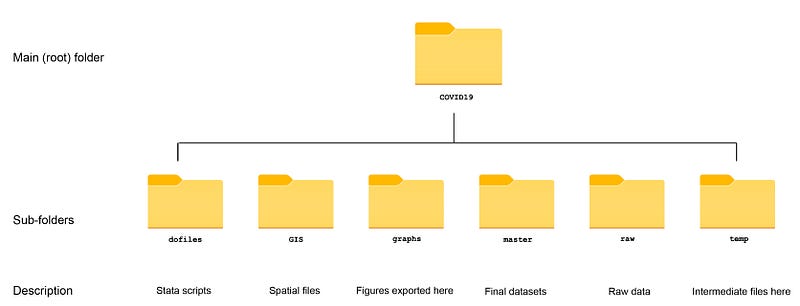
Within the graphs folder, I also create an additional sub-folder called guide6, to store the figures generated here. For details on how to organize your files, please see Guide 1.

In order to make the graphs exactly as they are shown here, several additional item are required:

• Install the cleanplots theme for a clean look for your figures (more on themes in Guide 2):

net install cleanplots, from("https://tdmize.github.io/data/cleanplots")

set scheme cleanplots, perm

• Install Ben Jann’s colorpalette package (more on colors in Guide 2 and in the Color guide)

net install palettes, replace from("https://raw.githubusercontent.com/benjann/palettes/master/")
net install colrspace, replace from("https://raw.githubusercontent.com/benjann/colrspace/master/")

• Set default graph font to Arial Narrow (see the Font guide on customizing fonts)

graph set window fontface "Arial Narrow"

This guide has been written in version 16.1 and should work with version 14 and onwards. Earlier versions might need some modification for implementing custom colors.

• This guide also requires the installation of FFmpeg, an open-source video-editing software. So make sure you have write permissions on the computer you are using.

Task 1: Get the data in order

The Oxford COVID-19 policy dataset was introduced and discussed extensively in Guide 3 including how to pull data from a Github repository. Therefore we will dive straight into setting up the data:

*** get the data
clear

insheet using "https://raw.githubusercontent.com/OxCGRT/covid-policy-tracker/master/data/OxCGRT_latest.csv", clear

*** new data has been added for USA and UK for regions so we drop the regions:
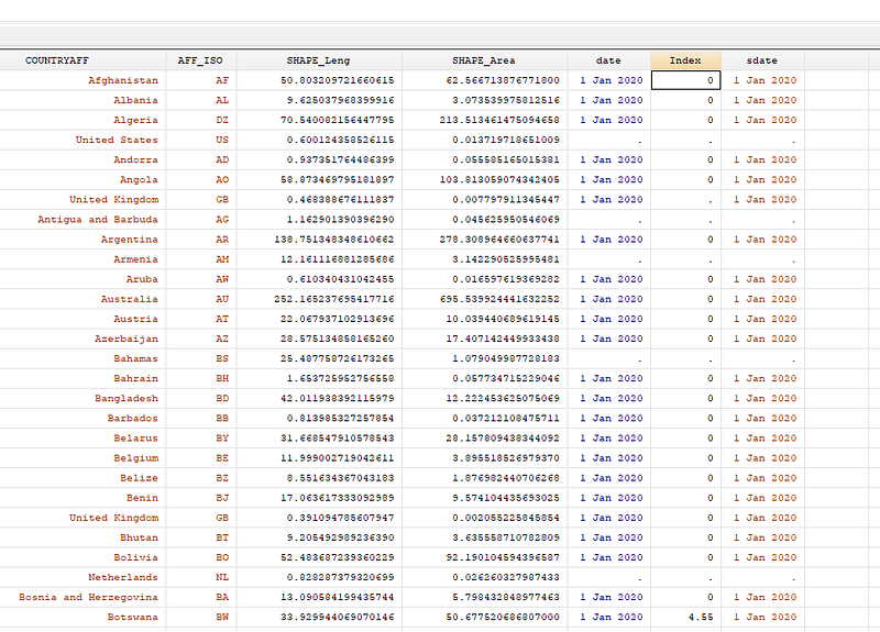
drop if regionname!=""

*** keep only the variables we need
keep date countryname containmenthealthindexfordisplay

ren containmenthealthindexfordisplay Index   // also used as a label
ren countryname country

duplicates list country date

*** fix the date

tostring date, gen(date2)    // string the date variable
drop date
gen date = date(date2,"YMD")
format date %tdDD-Mon-yyyy
drop date2
drop if date < 21915    // 1st January

order country date
sort country date

compress
save ./master/COVID_policies2.dta, replace

Here we keep the variables we need, fix the dates, and save the dataset in the master folder. Since we already generated a COVID_policies.dta dataset for the heatplots shown in Guide 3, therefore I label this dataset as COVID_policies2.dta.

Task 2: The map

Maps were discussed extensively in Guide 4 including where to find the shapefiles and set them up in Stata. To summarize, the shapefile for the world can be downloaded here, and saved and unzipped in the GIS folder.

The map setup, including dropping Antarctica and fixing the map projection, is done as follows:

********* get the shapefiles in order in order

cd GIS
spshape2dta "World_Countries__Generalized_.shp", replace saving(world)

*** set up the GIS files

use world_shp, clear
merge m:1 _ID using world 
 drop if COUNTRY=="Antarctica"
 drop rec_header- _merge
 geo2xy _Y _X, proj (web_mercator) replace
  sort _ID
  save, replace

In the next step, we merge the map data with the policies dataset after fixing some country names:

**** let's merge the datasets

use world, clear
 ren COUNTRY country
 drop if country=="Antarctica"

  
  
*** fix the names 
replace country="Cote d'Ivoire" if country=="Côte d'Ivoire"
replace country="Kyrgyz Republic" if country=="Kyrgyzstan"
replace country="Slovak Republic" if country=="Slovakia"
replace country="Democratic Republic of Congo" if country=="Congo DRC"
replace country="Russia" if country=="Russian Federation"
replace country="Palestine" if country=="Palestinian Territory"

*** merge with the policies database 

merge 1:m country using ../master/COVID_policies2
drop if _m==2
drop _m

Note that a bunch of small island states won’t match. They can be dealt with by merging them with another, more extensive map file. This is unfortunately a standard problem for these small islands as they tend to disappear in the sea of large countries. They are also hardly visible on global maps.

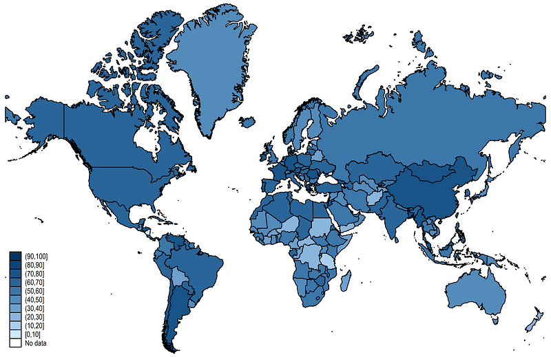
In the next step, we generate a basic map for the last date we have in the dataset and plot the HCI:

summ date
spmap Index using world_shp if date==`r(max)', ///
 id(_ID) clmethod(custom) clbreaks(0(10)100) fcolor(Blues2)

graph export ../graphs/animation/map1.png, replace wid(2000)

which gives us this default image:

The next code block, fine tunes this map by using a custom color scheme defined by the colorpalette package (introduced in Guide 2):

local date: display %tdd_m_yy date(c(current_date), "DMY")
display "`date'"

colorpalette matplotlib viridis, n(10) reverse nograph
local colors `r(p)'

summ date 
spmap Index using world_shp if date==`r(max)', ///
id(_ID) ///
clmethod(custom) clbreaks(0(10)100)  fcolor("`colors'")  ///
ocolor(white ..) osize(*0.15 ..)  ///
ndocolor(black) ndfcolor(gs14) ndlabel("No data")  ndsize(*0.15 ..)  ///
legend(pos(7) size(*0.8)) legstyle(2)  /// 
title("COVID-19 Policy Stringency Index (`date')", size(medium)) ///
   note("Data source: Oxford COVID-19 Government Response Tracker. Mercator projection used. Antartica dropped from maps." , size(*0.5))

graph export ../graphs/animation/map2.png, replace wid(2000)

In the code above, we auto generate the date and add it to the title. We also define the cut-offs in steps of ten, customize boundaries, no data zones, line widths etc. and get the following map:

In the graph above, the green shades in the middle HCI range are hard to differentiate, while the two yellowish tones, that show the bottom two categories, stand out a lot. The HCI range roughly between 20–50 is considered fairly weak on the aggregate level (individual dimensions of the index may still vary). It is only above 50 and 60 where one can consider policies to be strong, and above scores above 70 or 80 are considered to be very strong, well thought-out responses.

To highlight this point on the map, we can use a power shift to move the color tones around. This can be achieved through a manual interpolation of colors as follows:

colorpalette: matplotlib viridis, ipolate(10) name("Even") / ///
matplotlib viridis, ipolate(10, power(0.5)) name("Shift left") / ///
matplotlib viridis, ipolate(10, power(1.6)) name("Shift right")  

graph export ../graphs/animation/colorpalette.png, replace wid(2000)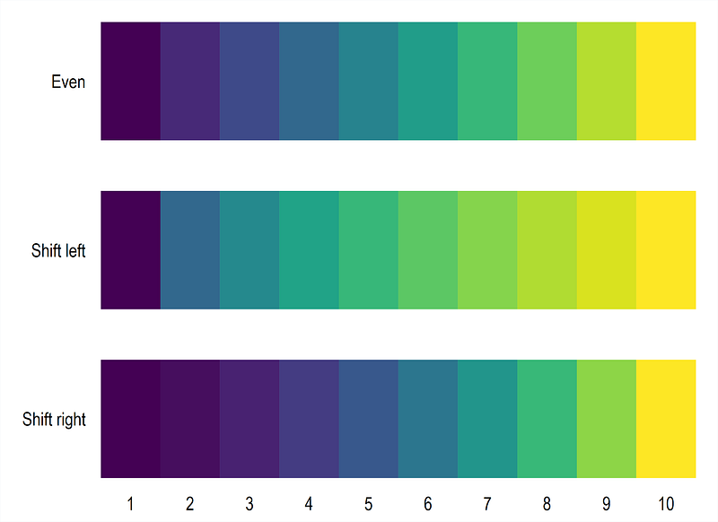

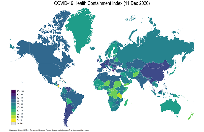
Here we see how the color interpolation changes relative to the evenly distributed color scheme. For our purposes, we will use the color bands labeled “Shift right” and redraw the map:

local date: display %tdd_m_yy date(c(current_date), "DMY")
display "`date'"     
     
colorpalette matplotlib viridis, ipolate(10, power(1.6)) reverse nograph
local colors `r(p)'

summ date 
spmap Index using world_shp if date==`r(max)', ///
id(_ID) ///
clmethod(custom) clbreaks(0(10)100)  fcolor("`colors'")  ///
ocolor(white ..) osize(*0.15 ..)  ///
ndocolor(black) ndfcolor(gs14) ndlabel("No data")  ndsize(*0.15 ..)  ///
legend(pos(7) size(*0.8)) legstyle(2)  /// 
title("COVID-19 Health Containment Index (`date')", size(medium)) ///
note("Data source: Oxford COVID-19 Government Response Tracker. Mercator projection used. Antartica dropped from maps." , size(*0.5))

graph export ../graphs/animation/map3.png, replace wid(2000)

which gives us this image:

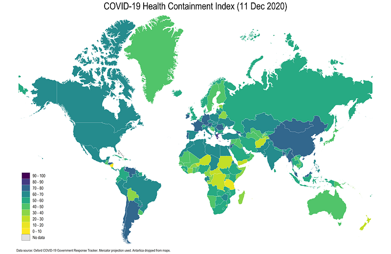
Here the policies are a bit more differentiated than the map with evenly distributed colors and the middle policy range countries are easier to identify.

Now that we have the color template in place, we need to generate the maps for each date. But before we loop over all the dates, we need to make sure that the dates are in a format such that they can be added in the title as well. This can be achieved in several different ways, but for this guide, we will do it using the custom labmask package:

ssc install labmask, replace  // install the custom package

gen sdate = string(date, "%tdd_m_yy") // define the date format
labmask date, values(sdate)  // mask the values

Here we generate a string variable called sdate, which has the dates in the correct display format. We then take this string variable and mask it on the date variable as value labels. This literally takes the string in each row and converts it to a label for a date variable:

We can now use this information to generate maps for each day using the following loop:

*** get the color scheme in place
colorpalette matplotlib viridis, ipolate(10, power(1.6)) reverse nograph
local colors `r(p)'

* here we recover the total number of dates
levelsof date, local(dates)

* main loop block
foreach x of local dates {

local t : label date `x'   // pick the date label in a local t
 display "`t'"

* main graph block:

spmap Index using world_shp if date==`x', ///
id(_ID) ///
clmethod(custom) clbreaks(0(10)100)  fcolor("`colors'")  ///
ocolor(white ..) osize(*0.15 ..)  ///
ndocolor(black) ndfcolor(gs14) ndlabel("No data")  ndsize(*0.15 ..)  ///
legend(pos(7) size(*0.8)) legstyle(2)  /// 
title("COVID-19 Health Containment Index (`t')", size(medium)) ///
 

* export each map as a fixed name + date
graph export "../graphs/guide6/HCI_`x'.png", replace wid(2000)  
   
}  // end of loop

Here we are doing exactly what we did in the previous step, except the if condition now says to pick the value of the date defined by the loop variable `x' . We are also using the value label of the date variable, stored in the local `t' for the map title.

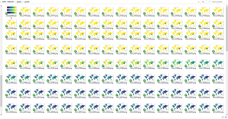
Once the loop is finished, a large set of files containing the maps will be generated in the guide6 folder. They all have a standardized name format: HCI_<date>.png.

Task 3: Making a video

In the next step, we need to combine the images to make a video. For this step, download the open-source software FFmpeg and click on the relevant operating system icon. The logos are marked below in red, since here the tendency is to click on the large green source code button:

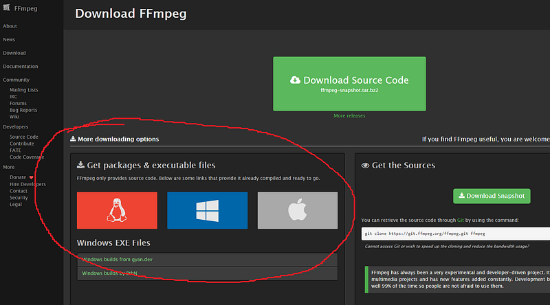
The documentation of FFmpeg is given here including all the commands that be used. FFmpeg is a syntax based software, without a GUI, so understanding all the options and possibilities also requires a good understanding of the commands available.

For Windows, clicking on the link above downloads a zipped file. This file can be extracted anywhere, for example, in some software folder, or even in the COVID19 folder defined above. I just copied it on my D: drive. What is really important is that you know the path of this folder for the next step:

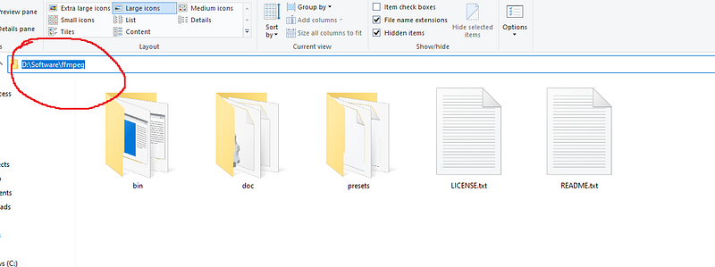
In Stata, we need define two globals to making the scripting easier. One for the directory path of FFmpeg which has to refer to the bin folder:

global ffmpegdir "D:/Software/ffmpeg/bin"  

global videodir  "D:/Programs/Dropbox/Dropbox/PROJECT COVID - MEDIUM/graphs/guide6"

The second global says where the video should be kept. Here I just keep the video folder same as the map images folder.

We can now use the following syntax to generate the video:

! "$ffmpegdir/ffmpeg.exe" -y -framerate 10 -start_number 21915 -i "$videodir/HCI_%02d.png" -c:v libx264 -crf 15 -r 30 "$videodir/Video.mp4"

In this code, several FFmpeg options are used. While we won’t discuss all of these, the key ones are as follows:

! tells Stata to load the Windows command shell

-y is the default DOS command for replacing files (if you learned programming in the 1980s, this would be obvious :))

-framerate 10 says how many frames per second. If this is reduced then the video is slower.

-start_number 21915 says, which is the file number to start with. This should be the number given at the end of the first file.

-i says to read all the files which match the criteria HCI_%02d.png

The remaining options are codecs that generates the video. For example -crf is constant rate factor. Here a lower crf value will give a higher quality. 0 is for lossless animation, but it will also produce a larger file. Usually values in the range of 5–15 are good options.

-r is the output framerate option, which is different from the -framerate command defined earlier. Both can be used to control the speed of the animation.

If the above syntax is correctly specified, and both FFmmpeg and image paths are correct, then a screen should pop up which should show an output like this:

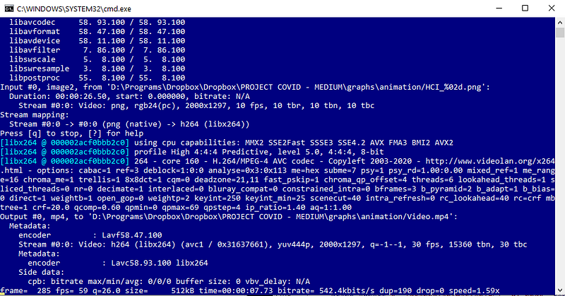
If something is wrong with the syntax, then nothing will happen. At the end of the execution, a file named video.mp4 will be created in the specified folder. Here I will go an additional step and filter it again:

! "$ffmpegdir/ffmpeg.exe" -y -i "$videodir/Video.mp4" -filter "minterpolate='mi_mode=blend:fps=120'" "$videodir/Video_smooth.mp4"

The step above, creates a smooth transition between frames so it looks less jerky. Again this is something to experiment with, but here we get the final video_smooth.mp4 file which looks like this:

The steps explained above, can be applied to any Stata animation, and not just maps. As long as there is a good control over colors, axes, legends, file naming conventions etc., anything can be animated. For other examples, you can also visit my YouTube channel to check out various sample Stata animations.

NOTE: the guide was updated in Dec 2020 to fix some links and make the code a bit more efficient. Therefore the figures were updated but the video file on YouTube remains the same.

Exercise

Try generating a map with another policy variable, try other color schemes, and experiment with different FFmpeg options. Try and also animate a line graph or distributions over time.

Other Stata guides

Part 1: An introduction to data setup and customized graphs

Part 2: Customizing colors schemes

Part 3: Heat plots

Part 4: Maps

Part 5: Stacked area graphs

Part 6: Animations

Part 7: Doubling time graphs I

Part 8: Ridge-line plots (Joy plots)

Part 9: Customized bar graphs

Part 10: Stream graphs

If you enjoy these guides and find them useful, then please like and follow The Stata Guide. Also, please share your visualizations if you use these guides!

About the author

I am an economist by profession and I have been using Stata since 2003. I am currently based in Vienna, Austria where I work at the Vienna University of Economics and Business (WU) and at the International Institute for Applied Systems Analysis (IIASA). You can find my research work on ResearchGate and Google Scholar, and Stata code repository on GitHub. You can follow my COVID-19 related Stata visualizations on my Twitter. I am also featured on the Stata COVID-19 webpage in the visualization and graphics section.

You can connect with me via Medium, Twitter, LinkedIn or simply via email: [email protected].

My Medium blog for Stata stuff here: The Stata Guide where new awesome content is released regularly. Clap, and/or follow if you like these guides!