Implemented Neural Networks Projects

Repo for all the projects ( vertical post)…

Welcome back peeps.

Since we are now focusing on our goals for 2023 — new vertical series than horizontal ( means you will find all the contents of the series in one post and projects in second than developing/extending it to new posts every time). So, keep checking this post every day to see new projects.

Prerequisite to these projects —

Complete 60 days of Data Science and Machine Learning before starting this series ( link below) —

Day 1 — Day 60 : Quick Recap of 60 days of Data Science and ML

Connect the ML dots…

medium.com

Projects Videos —

Subscribe today!

Ignito

Excited to share that we have launched our Youtube channel — Ignito to cover all the projects and coding exercise for …

www.youtube.com

Tech Newsletter —

If you are interested, you can join my newsletter through which I send tech interview tips, techniques, patterns, hacks — Software Development, ML, Data Science, Startups and Technology projects to more than 35K readers. You can subscribe to Ignito:

Ignito

Data Science, ML, AI and more… Click to read Ignito, by Naina Chaturvedi, a Substack publication with hundreds of…

naina0405.substack.com

Let’s dive in!

A neural network is a type of machine learning algorithm modeled after the structure and function of the human brain. It is composed of layers of interconnected “neurons,” which process and transmit information.

In a neural network, input data is passed through multiple layers of neurons, each of which applies a mathematical operation to the data. These operations, called “weights,” are learned by the network through a process called training.

The output of the final layer is then used to make predictions or decisions. The network can be trained using a labeled dataset, where the desired output is known for a given input, and the network’s weights are adjusted to minimize the difference between its output and the desired output.

import numpy as np

# Define the sigmoid activation function
def sigmoid(x):
    return 1 / (1 + np.exp(-x))

# Define the derivative of the sigmoid function
def sigmoid_derivative(x):
    return sigmoid(x) * (1 - sigmoid(x))

# Define the neural network class
class NeuralNetwork:
    def __init__(self, input_dim, hidden_dim, output_dim):
        # Initialize the weights and biases with random values
        self.W1 = np.random.randn(hidden_dim, input_dim)
        self.b1 = np.random.randn(hidden_dim, 1)
        self.W2 = np.random.randn(output_dim, hidden_dim)
        self.b2 = np.random.randn(output_dim, 1)

    def forward_propagation(self, X):
        # Perform forward propagation
        self.Z1 = np.dot(self.W1, X) + self.b1
        self.A1 = sigmoid(self.Z1)
        self.Z2 = np.dot(self.W2, self.A1) + self.b2
        self.A2 = sigmoid(self.Z2)

    def backward_propagation(self, X, y):
        # Perform backward propagation and update the weights and biases
        m = X.shape[1]
        dZ2 = self.A2 - y
        dW2 = (1 / m) * np.dot(dZ2, self.A1.T)
        db2 = (1 / m) * np.sum(dZ2, axis=1, keepdims=True)
        dZ1 = np.dot(self.W2.T, dZ2) * sigmoid_derivative(self.Z1)
        dW1 = (1 / m) * np.dot(dZ1, X.T)
        db1 = (1 / m) * np.sum(dZ1, axis=1, keepdims=True)

        self.W2 -= learning_rate * dW2
        self.b2 -= learning_rate * db2
        self.W1 -= learning_rate * dW1
        self.b1 -= learning_rate * db1

    def train(self, X, y, epochs):
        for epoch in range(epochs):
            self.forward_propagation(X)
            self.backward_propagation(X, y)

    def predict(self, X):
        self.forward_propagation(X)
        return self.A2

# Example usage
X_train = np.array([[0, 0], [0, 1], [1, 0], [1, 1]]).T
y_train = np.array([[0, 1, 1, 0]])

# Define the hyperparameters
input_dim = 2
hidden_dim = 2
output_dim = 1
learning_rate = 0.1
epochs = 10000

# Create a neural network instance
nn = NeuralNetwork(input_dim, hidden_dim, output_dim)

# Train the neural network
nn.train(X_train, y_train, epochs)

# Make predictions
X_test = np.array([[0, 0], [0, 1], [1, 0], [1, 1]]).T
predictions = nn.predict(X_test)
print(predictions)

In this code snippet, we define a simple neural network class (NeuralNetwork) with a constructor that initializes the weights and biases randomly. The class has methods for forward propagation (forward_propagation) and backward propagation (backward_propagation) to update the weights and biases based on the computed errors. The train method is used to train the network by performing forward and backward propagation for a specified number of epochs. The predict method is used to make predictions using the trained network.

In the example usage part, we create a simple XOR dataset (X_train and y_train) for training. We define the hyperparameters such as the input dimension, hidden dimension, output dimension, learning rate, and the number of epochs.

We then create an instance of the NeuralNetwork class with the specified dimensions. Next, we train the network by calling the train method and passing the training data and the number of epochs. During training, the network performs forward propagation, computes the errors using backward propagation, and updates the weights and biases.

After training, we can use the predict method to make predictions on new data (X_test). The predictions are stored in the predictions variable, which we print to see the predicted output.

There are several types of neural networks, including feedforward networks, which pass the input data through the layers in one direction, and recurrent networks, which allow for feedback connections and can process sequential data.

import tensorflow as tf
from tensorflow.keras.models import Sequential
from tensorflow.keras.layers import Dense

# Define the neural network architecture
model = Sequential([
    Dense(64, activation='relu', input_shape=(input_dim,)),
    Dense(64, activation='relu'),
    Dense(num_classes, activation='softmax')
])

# Compile the model
model.compile(optimizer='adam',
              loss='categorical_crossentropy',
              metrics=['accuracy'])

# Train the model
model.fit(X_train, y_train, epochs=10, batch_size=32)

# Evaluate the model
loss, accuracy = model.evaluate(X_test, y_test)
print(f'Test loss: {loss:.4f}')
print(f'Test accuracy: {accuracy:.4f}')

# Make predictions using the trained model
predictions = model.predict(X_new)

We import the necessary libraries, including TensorFlow and the required modules from Keras.
We define the neural network architecture using the Sequential class from Keras. This architecture consists of three dense (fully connected) layers. The first two layers have 64 units with the ReLU activation function, and the last layer has the number of units equal to the number of classes in the classification task with the softmax activation function.
We compile the model by specifying the optimizer, loss function, and metrics to be used during training.
We train the model using the fit method, passing the training data (X_train and y_train) along with the number of epochs and batch size.
We evaluate the trained model on the test data (X_test and y_test) using the evaluate method and print the test loss and accuracy.
Finally, we make predictions using the trained model on new data (X_new) using the predict method.

Deep neural networks, which have multiple layers, are able to learn and represent very complex patterns in the data and are widely used in computer vision, natural language processing, speech recognition and other fields.

This post will house all the Neural Networks projects related to the topics below-

Neural Networks

Neural Networks basics

Different types of neural networks

Linear Classifiers

Optimization

Hyper Parameter Tuning

Gradient Descent

Backpropagation Algorithm

Regularization — L2 and dropout regularization

Batch normalization

Build a neural network in Keras

Build a Neural Network With Pytorch

Build a neural network in TensorFlow

Train Neural Networks

Feedforward neural network

Popular Optimization Algorithms

Activation Functions

Strategies for reducing errors

Shallow Neural Networks

Convolutional Neural Networks

Convolution basics and CNN Architectures

Residual networks

Build a Convolutional Network

Batch Normalization and Dropout

Recurrent Neural Networks

RNN Basics

LSTM: Long Short Term Memory Cells

Natural language processing and Word Embeddings

Tensorflow

Tensorflow basics

Tensorflow Playground

Custom Loss Functions

Custom Layers and Models

Callbacks

Distributed Training

Data Pipelines with TensorFlow Data Services

Performance

Autoencoders

Autoencoders Basics

Generative Learning

Generative Adversarial Networks

Generative Adversarial Networks Basics

Useful activation functions and Batch normalization

Transposed convolutions

Generator and Discriminator

Deep Convolutional Generative Adversarial Networks

Implement Generative Adversarial Networks

Attention and Transformers

Attention and Transformers Basics

Sequence to Sequence Models

Attention

Multi-Head Self-Attention

Building Blocks of Transformers

Encoder

Decoder

Parameters Sharing

Build a Transformer Encoder

Graph Neural Networks

Basics of Graphs

Graph Convolutional Networks

Implement — Graph Convolutional Network

Natural Language Processing

Natural Language Processing Basics

Probabilistic Models

Sequence Models

Attention Models

First we will cover above mentioned topics in detail as follows —

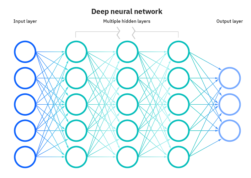
Neural Networks

Neural Networks basics

Neural networks are a fundamental component of deep learning, a subfield of machine learning. A neural network is a computational model inspired by the structure and functioning of biological neural networks, such as the human brain. It consists of interconnected artificial neurons, also known as nodes or units, organized into layers.

The basic building block of a neural network is the artificial neuron or node. Each neuron takes in one or more input values, performs a weighted sum of these inputs, applies an activation function to the sum, and produces an output. The activation function introduces non-linearity into the network, enabling it to model complex relationships between inputs and outputs.

Neurons in a neural network are organized into layers. Typically, a neural network has an input layer, one or more hidden layers, and an output layer. The input layer receives the input data, and the output layer produces the final output or prediction. The hidden layers are intermediary layers between the input and output layers and play a crucial role in learning complex patterns and representations.

Deep learning refers to the use of neural networks with multiple hidden layers. Deep neural networks are capable of automatically learning hierarchical representations of data. Each layer in a deep neural network extracts higher-level features from the representations learned by the previous layer. This enables the network to learn more abstract and complex representations as the depth increases.

Training a neural network involves a process called backpropagation, which is based on the gradient descent optimization algorithm. During training, the network adjusts its weights and biases based on the errors between the predicted outputs and the true outputs. This iterative process continues until the network’s performance reaches a satisfactory level.

import numpy as np

# Define the sigmoid activation function
def sigmoid(x):
    return 1 / (1 + np.exp(-x))

# Define the derivative of the sigmoid function
def sigmoid_derivative(x):
    return sigmoid(x) * (1 - sigmoid(x))

# Define the neural network class
class NeuralNetwork:
    def __init__(self, input_dim, hidden_dim, output_dim):
        # Initialize the weights and biases with random values
        self.W1 = np.random.randn(hidden_dim, input_dim)
        self.b1 = np.random.randn(hidden_dim, 1)
        self.W2 = np.random.randn(output_dim, hidden_dim)
        self.b2 = np.random.randn(output_dim, 1)

    def forward_propagation(self, X):
        # Perform forward propagation
        self.Z1 = np.dot(self.W1, X) + self.b1
        self.A1 = sigmoid(self.Z1)
        self.Z2 = np.dot(self.W2, self.A1) + self.b2
        self.A2 = sigmoid(self.Z2)

    def backward_propagation(self, X, y):
        # Perform backward propagation and update the weights and biases
        m = X.shape[1]
        dZ2 = self.A2 - y
        dW2 = (1 / m) * np.dot(dZ2, self.A1.T)
        db2 = (1 / m) * np.sum(dZ2, axis=1, keepdims=True)
        dZ1 = np.dot(self.W2.T, dZ2) * sigmoid_derivative(self.Z1)
        dW1 = (1 / m) * np.dot(dZ1, X.T)
        db1 = (1 / m) * np.sum(dZ1, axis=1, keepdims=True)

        self.W2 -= learning_rate * dW2
        self.b2 -= learning_rate * db2
        self.W1 -= learning_rate * dW1
        self.b1 -= learning_rate * db1

    def train(self, X, y, epochs):
        for epoch in range(epochs):
            self.forward_propagation(X)
            self.backward_propagation(X, y)

    def predict(self, X):
        self.forward_propagation(X)
        return self.A2

# Example usage
X_train = np.array([[0, 0], [0, 1], [1, 0], [1, 1]]).T
y_train = np.array([[0, 1, 1, 0]])

# Define the hyperparameters
input_dim = 2
hidden_dim = 2
output_dim = 1
learning_rate = 0.1
epochs = 10000

# Create a neural network instance
nn = NeuralNetwork(input_dim, hidden_dim, output_dim)

# Train the neural network
nn.train(X_train, y_train, epochs)

# Make predictions
X_test = np.array([[0, 0], [0, 1], [1, 0], [1, 1]]).T
predictions = nn.predict(X_test)
print(predictions)

We define the sigmoid activation function and its derivative. The sigmoid function is used as the activation function for the neurons in the network.
We define the NeuralNetwork class, which represents a simple feedforward neural network. The constructor initializes the weights and biases with random values.
The forward_propagation method performs forward propagation through the network, computing the outputs of each layer using the
The backward_propagation method performs backward propagation through the network, calculating the gradients of the weights and biases and updating them based on the computed errors. This step is essential for training the network.
The train method is used to train the neural network. It iterates over the specified number of epochs and performs forward and backward propagation to update the weights and biases based on the training data.
The predict method performs forward propagation on new data to make predictions using the trained network.
In the example usage part, we define a simple XOR dataset (X_train and y_train) for training.
We define the hyperparameters such as the input dimension, hidden dimension, output dimension, learning rate, and the number of epochs.
We create an instance of the NeuralNetwork class with the specified dimensions.
We train the neural network by calling the train method and passing the training data and the number of epochs. During training, the network updates the weights and biases based on the computed errors.
After training, we can use the predict method to make predictions on new data (X_test). The predictions are stored in the predictions variable, which we print to see the predicted output.

Different types of neural networks

Feedforward Neural Networks (FNN): Also known as multi-layer perceptrons (MLPs), feedforward neural networks are the most basic type. They consist of an input layer, one or more hidden layers, and an output layer. The information flows only in one direction, from the input layer through the hidden layers to the output layer. FNNs are used for tasks like classification and regression.
Convolutional Neural Networks (CNN): CNNs are primarily designed for image and video processing. They employ specialized layers called convolutional layers that apply convolution operations to input data. These layers enable the network to automatically learn hierarchical representations of visual data. CNNs have been highly successful in image classification, object detection, and image segmentation tasks.
Recurrent Neural Networks (RNN): RNNs are designed to handle sequential data, such as time series or natural language. They introduce loops in the network architecture, allowing information to persist and be shared across different time steps. This enables RNNs to capture temporal dependencies in the data. Long Short-Term Memory (LSTM) and Gated Recurrent Unit (GRU) are popular variations of RNNs that address the vanishing gradient problem and improve the ability to capture long-term dependencies.
Generative Adversarial Networks (GAN): GANs consist of two components: a generator network and a discriminator network. The generator network generates synthetic data samples, such as images, while the discriminator network tries to distinguish between real and generated data. GANs are used for tasks like image generation, style transfer, and data augmentation.
Autoencoders: Autoencoders are unsupervised learning models that aim to learn efficient representations of the input data. They consist of an encoder network that compresses the input data into a lower-dimensional representation, and a decoder network that reconstructs the original input from the compressed representation. Autoencoders can be used for tasks like data denoising, dimensionality reduction, and anomaly detection.
Recursive Neural Networks (Tree-based Neural Networks): These neural networks operate on hierarchical structures like parse trees or constituency trees. They capture dependencies and relationships among elements in the tree structure. Recursive neural networks are commonly used in natural language processing tasks, such as sentiment analysis and parsing.

Implementation —

import numpy as np
import tensorflow as tf
from tensorflow.keras.models import Sequential
from tensorflow.keras.layers import Dense, Conv2D, MaxPooling2D, LSTM

# Example usage
X_train = np.random.randn(1000, 784)  # Example input data (1000 samples, 784 features)
y_train = np.random.randint(0, 10, size=(1000,))  # Example labels (1000 samples, 10 classes)

# Define hyperparameters
input_dim = 784
num_classes = 10
height, width, channels = 28, 28, 1
sequence_length = 20
learning_rate = 0.001
epochs = 10

# Feedforward Neural Network
def create_feedforward_network():
    model = Sequential([
        Dense(64, activation='relu', input_shape=(input_dim,)),
        Dense(64, activation='relu'),
        Dense(num_classes, activation='softmax')
    ])
    return model

# Convolutional Neural Network (CNN)
def create_cnn():
    model = Sequential([
        Conv2D(32, kernel_size=(3, 3), activation='relu', input_shape=(height, width, channels)),
        MaxPooling2D(pool_size=(2, 2)),
        Conv2D(64, kernel_size=(3, 3), activation='relu'),
        MaxPooling2D(pool_size=(2, 2)),
        Dense(64, activation='relu'),
        Dense(num_classes, activation='softmax')
    ])
    return model

# Recurrent Neural Network (RNN)
def create_rnn():
    model = Sequential([
        LSTM(64, input_shape=(sequence_length, input_dim)),
        Dense(num_classes, activation='softmax')
    ])
    return model

# Create a feedforward neural network
feedforward_model = create_feedforward_network()
feedforward_model.compile(optimizer='adam',
                          loss='sparse_categorical_crossentropy',
                          metrics=['accuracy'])
feedforward_model.fit(X_train, y_train, epochs=epochs)

# Create a CNN
cnn_model = create_cnn()
cnn_model.compile(optimizer='adam',
                  loss='sparse_categorical_crossentropy',
                  metrics=['accuracy'])
cnn_model.fit(X_train, y_train, epochs=epochs)

# Create an RNN
rnn_model = create_rnn()
rnn_model.compile(optimizer='adam',
                  loss='sparse_categorical_crossentropy',
                  metrics=['accuracy'])
rnn_model.fit(X_train, y_train, epochs=epochs)

In this code, I have provided random example input data (X_train) and labels (y_train) for demonstration purposes. You can replace them with your own dataset.

The hyperparameters such as input_dim (input dimension), num_classes (number of classes), height, width, channels (image dimensions), sequence_length (length of input sequences for RNN), learning_rate, and epochs can be modified according to your specific task and dataset.

The code then creates instances of the feedforward neural network, CNN, and RNN by calling the respective functions (create_feedforward_network, create_cnn, create_rnn). Each model is compiled with the appropriate optimizer, loss function, and metrics.

Finally, the models are trained using the fit method, where the training data (X_train and y_train) and the number of epochs are passed as arguments.

Linear Classifiers

Linear classifiers are a type of machine learning algorithm used for classification tasks. They make predictions based on a linear combination of the input features, often referred to as features’ weights or coefficients. Linear classifiers aim to separate data points belonging to different classes by finding an optimal linear decision boundary.

One commonly used linear classifier is the Support Vector Machine (SVM). SVM seeks to find the best hyperplane that maximally separates the data points of different classes.

Implementation —

from sklearn import datasets
from sklearn.model_selection import train_test_split
from sklearn.svm import SVC
from sklearn.metrics import accuracy_score

# Load the Iris dataset
iris = datasets.load_iris()
X = iris.data  # Input features
y = iris.target  # Target variable

# Split the dataset into training and testing sets
X_train, X_test, y_train, y_test = train_test_split(X, y, test_size=0.2, random_state=42)

# Create a linear classifier (SVM)
svm = SVC(kernel='linear')

# Train the classifier
svm.fit(X_train, y_train)

# Make predictions on the test set
y_pred = svm.predict(X_test)

# Calculate the accuracy of the classifier
accuracy = accuracy_score(y_test, y_pred)
print("Accuracy:", accuracy)

We import the necessary libraries, including datasets from sklearn to load the Iris dataset, train_test_split to split the data into training and testing sets, SVC from sklearn.svm to create a support vector machine classifier, and accuracy_score from sklearn.metrics to evaluate the classifier's accuracy.
The Iris dataset is loaded, where X represents the input features and y represents the target variable.
The dataset is split into training and testing sets using the train_test_split function from sklearn.model_selection.
We create an instance of the SVC class, which represents a support vector machine classifier with a linear kernel.
The classifier is trained on the training data using the fit method.
Predictions are made on the test set using the predict method.
The accuracy of the classifier is calculated by comparing the predicted labels (y_pred) with the true labels (y_test).
Finally, the accuracy is printed.

Optimization and Hyper Parameter Tuning

Optimization refers to the process of finding the best set of parameters or configurations that minimize or maximize an objective function. In machine learning, optimization is used to train models by adjusting the parameters to minimize the loss function and improve performance.

Hyperparameter tuning, on the other hand, is the process of finding the best values for the hyperparameters of a machine learning model. Hyperparameters are settings that are not learned from the data but are set by the user before training the model. Examples of hyperparameters include learning rate, number of hidden layers, regularization strength, and batch size.

One commonly used method for hyperparameter tuning is grid search, which exhaustively searches through a predefined set of hyperparameters and evaluates the model’s performance for each combination.

Implementation —

from sklearn import datasets
from sklearn.model_selection import train_test_split, GridSearchCV
from sklearn.svm import SVC
from sklearn.metrics import accuracy_score

# Load the Iris dataset
iris = datasets.load_iris()
X = iris.data  # Input features
y = iris.target  # Target variable

# Split the dataset into training and testing sets
X_train, X_test, y_train, y_test = train_test_split(X, y, test_size=0.2, random_state=42)

# Define the hyperparameters to tune
hyperparameters = {
    'C': [0.1, 1, 10],
    'kernel': ['linear', 'rbf'],
    'gamma': [0.1, 1, 10]
}

# Create a classifier (SVM)
svm = SVC()

# Perform grid search to find the best hyperparameters
grid_search = GridSearchCV(svm, hyperparameters, scoring='accuracy', cv=5)
grid_search.fit(X_train, y_train)

# Get the best hyperparameters and model
best_params = grid_search.best_params_
best_model = grid_search.best_estimator_

# Make predictions on the test set using the best model
y_pred = best_model.predict(X_test)

# Calculate the accuracy of the best model
accuracy = accuracy_score(y_test, y_pred)
print("Best Hyperparameters:", best_params)
print("Accuracy:", accuracy)

We import the necessary libraries, including datasets from sklearn to load the Iris dataset, train_test_split to split the data into training and testing sets, SVC from sklearn.svm to create a support vector machine classifier, GridSearchCV from sklearn.model_selection for performing grid search, and accuracy_score from sklearn.metrics to evaluate the model's accuracy.
The Iris dataset is loaded, where X represents the input features and y represents the target variable.
The dataset is split into training and testing sets using the train_test_split function from sklearn.model_selection.
We define a dictionary hyperparameters that contains the hyperparameters to tune. In this example, we tune the C parameter, kernel, and gamma for the SVM classifier.
We create an instance of the SVM classifier.
Grid search is performed using the GridSearchCV class, where we pass the classifier, hyperparameters, scoring metric (accuracy in this case), and the number of folds for cross-validation (cv=5).
The grid search is performed by calling the fit method on the training data.
We retrieve the best hyperparameters and the best model from the grid search results.
Predictions are made on the test set using the best model.

Gradient Descent

Gradient Descent is an iterative optimization algorithm used to minimize the cost function of a machine learning model. It is commonly used in training models by adjusting the parameters iteratively to find the optimal values that minimize the difference between the predicted and actual outputs.

The basic idea behind Gradient Descent is to update the parameters in the direction of the steepest descent of the cost function. It calculates the gradient of the cost function with respect to each parameter and takes steps proportional to the negative of the gradient to reach the minimum.

Implementation —

import numpy as np
import matplotlib.pyplot as plt

# Generate random data
np.random.seed(42)
X = np.random.rand(100, 1)
y = 4 + 3 * X + np.random.randn(100, 1)

# Add bias term to X
X_b = np.c_[np.ones((100, 1)), X]

# Define the learning rate and number of iterations
learning_rate = 0.1
n_iterations = 1000

# Initialize the parameters
theta = np.random.randn(2, 1)

# Perform Gradient Descent
for iteration in range(n_iterations):
    gradients = 2 / 100 * X_b.T.dot(X_b.dot(theta) - y)
    theta = theta - learning_rate * gradients

# Print the final parameters
print("Intercept:", theta[0][0])
print("Slope:", theta[1][0])

# Plot the data and fitted line
plt.scatter(X, y)
plt.plot(X, X_b.dot(theta), color='red')
plt.xlabel("X")
plt.ylabel("y")
plt.show()

We generate random data X and corresponding labels y using np.random.rand and adding Gaussian noise.
We add a bias term to X by concatenating a column of ones to the left of X using np.c_.
We define the learning rate and number of iterations.
The parameters theta are initialized randomly.
We perform Gradient Descent by iterating over the specified number of iterations. In each iteration, we calculate the gradients using the formula gradients = 2 / 100 * X_b.T.dot(X_b.dot(theta) - y) and update the parameters using theta = theta - learning_rate * gradients.
After the iterations, we print the final values of the parameters.
Finally, we plot the data points using plt.scatter and the fitted line using plt.plot to visualize the results.

Back-propagation Algorithm

Backpropagation is an algorithm used to train neural networks with multiple layers. It calculates the gradient of the loss function with respect to the weights and biases in the network, allowing for efficient updates of these parameters during the training process.

The backpropagation algorithm involves two main steps: forward propagation and backward propagation.

During forward propagation, the input data is fed through the network, and the activations of each layer are calculated sequentially. These activations are then used to compute the network’s output.

During backward propagation, the error between the predicted output and the true output is calculated. This error is then backpropagated through the network, layer by layer, to calculate the gradients of the weights and biases. These gradients are used to update the parameters in order to minimize the error.

import numpy as np

# Define the sigmoid activation function and its derivative
def sigmoid(x):
    return 1 / (1 + np.exp(-x))

def sigmoid_derivative(x):
    return sigmoid(x) * (1 - sigmoid(x))

# Define the neural network class
class NeuralNetwork:
    def __init__(self, input_dim, hidden_dim, output_dim):
        self.input_dim = input_dim
        self.hidden_dim = hidden_dim
        self.output_dim = output_dim

        # Initialize the weights and biases randomly
        self.weights1 = np.random.randn(self.input_dim, self.hidden_dim)
        self.biases1 = np.zeros((1, self.hidden_dim))
        self.weights2 = np.random.randn(self.hidden_dim, self.output_dim)
        self.biases2 = np.zeros((1, self.output_dim))

    def forward_propagation(self, X):
        # Calculate the activations of the hidden layer
        self.hidden_activations = sigmoid(np.dot(X, self.weights1) + self.biases1)

        # Calculate the output of the network
        self.output = sigmoid(np.dot(self.hidden_activations, self.weights2) + self.biases2)

    def backward_propagation(self, X, y):
        # Calculate the error and delta of the output layer
        error = y - self.output
        delta_output = error * sigmoid_derivative(self.output)

        # Calculate the error and delta of the hidden layer
        hidden_error = delta_output.dot(self.weights2.T)
        delta_hidden = hidden_error * sigmoid_derivative(self.hidden_activations)

        # Update the weights and biases using the gradients
        self.weights2 += self.hidden_activations.T.dot(delta_output)
        self.biases2 += np.sum(delta_output, axis=0, keepdims=True)
        self.weights1 += X.T.dot(delta_hidden)
        self.biases1 += np.sum(delta_hidden, axis=0, keepdims=True)

    def train(self, X, y, epochs):
        for epoch in range(epochs):
            self.forward_propagation(X)
            self.backward_propagation(X, y)

    def predict(self, X):
        self.forward_propagation(X)
        return self.output

# Example usage
X = np.array([[0, 0], [0, 1], [1, 0], [1, 1]])
y = np.array([[0], [1], [1], [0]])

# Create a neural network with 2 input units, 2 hidden units, and 1 output unit
nn = NeuralNetwork(2, 2, 1)

# Train the neural network
nn.train(X, y, epochs=10000)

# Make predictions
predictions = nn.predict(X)
print("Predictions:")
print(predictions)

The sigmoid activation function and its derivative are defined. The sigmoid function returns the output of the sigmoid activation, which is calculated as 1 / (1 + exp(-x)). The sigmoid_derivative function computes the derivative of the sigmoid function.
The code then defines the NeuralNetwork class, which represents a simple feedforward neural network. The constructor method initializes the network’s dimensions, weights, and biases. The weights are initialized randomly using numpy’s randn function, and the biases are set to zeros.
The forward_propagation method performs the forward pass through the network. It calculates the activations of the hidden layer by applying the sigmoid activation function to the weighted sum of the input and biases. Then, it computes the output of the network by applying the sigmoid activation function to the weighted sum of the hidden layer activations and biases.
The backward_propagation method calculates the error between the predicted output and the true output. It then computes the deltas (gradients) of the output and hidden layers using the error and the derivative of the sigmoid function. The weights and biases are updated using these deltas and the activations from the forward pass.
The train method performs the training process by iterating over a specified number of epochs. It calls the forward_propagation and backward_propagation methods to update the weights and biases based on the computed errors.
The predict method performs forward propagation to obtain the output of the network given an input.

Regularization — L2 and dropout regularization

Regularization is a technique used to prevent overfitting in machine learning models by adding a penalty term to the loss function. It helps control the complexity of the model and reduces the impact of irrelevant features.

L2 regularization, also known as Ridge regularization, is a common regularization technique that adds a penalty term proportional to the sum of the squared weights to the loss function. This penalty encourages the model to have smaller weight values, which helps prevent overfitting. The regularization term is controlled by a hyperparameter called the regularization parameter (lambda).

Dropout regularization is a technique that randomly drops out a fraction of the neurons in a neural network during training. This helps prevent overfitting by introducing redundancy and reducing the co-adaptation of neurons. During prediction, all neurons are used, but their outputs are scaled to compensate for the dropout during training.

import numpy as np
from sklearn.datasets import make_classification
from sklearn.model_selection import train_test_split
from sklearn.linear_model import LogisticRegression
from sklearn.metrics import accuracy_score

# Generate a random classification dataset
X, y = make_classification(n_samples=1000, n_features=10, random_state=42)

# Split the dataset into training and testing sets
X_train, X_test, y_train, y_test = train_test_split(X, y, test_size=0.2, random_state=42)

# Apply L2 regularization (Ridge regularization)
logreg = LogisticRegression(penalty='l2', C=1.0)
logreg.fit(X_train, y_train)

# Make predictions on the test set
y_pred = logreg.predict(X_test)

# Calculate the accuracy
accuracy = accuracy_score(y_test, y_pred)
print("Accuracy with L2 regularization:", accuracy)

# Apply dropout regularization
class NeuralNetwork:
    def __init__(self, dropout_rate=0.5):
        self.dropout_rate = dropout_rate
        self.weights = None

    def fit(self, X, y):
        # Apply dropout during training
        if self.dropout_rate > 0:
            dropout_mask = np.random.binomial(1, 1 - self.dropout_rate, size=X.shape)
            X *= dropout_mask
            X /= 1 - self.dropout_rate

        # Train the model
        self.weights = np.linalg.inv(X.T.dot(X)).dot(X.T).dot(y)

    def predict(self, X):
        # No dropout during prediction
        return np.dot(X, self.weights)

# Create a neural network with dropout regularization
nn = NeuralNetwork(dropout_rate=0.5)

# Fit the neural network to the training data
nn.fit(X_train, y_train)

# Make predictions on the test set
y_pred = nn.predict(X_test)

# Convert predicted probabilities to class labels
y_pred = np.round(y_pred)

# Calculate the accuracy
accuracy = accuracy_score(y_test, y_pred)
print("Accuracy with dropout regularization:", accuracy)

We generate a random classification dataset using make_classification from sklearn.datasets.
The dataset is split into training and testing sets using train_test_split from sklearn.model_selection.
L2 regularization is applied using LogisticRegression from sklearn.linear_model, by setting the penalty parameter to 'l2'.
Predictions are made on the test set using the trained logistic regression model.
The accuracy of the model with L2 regularization is calculated using accuracy_score from sklearn.metrics.
Dropout regularization is implemented in a custom NeuralNetwork class. During training, a dropout mask is applied to the input data. The dropout mask is created using np.random.binomial to randomly set elements to 0 based on the dropout rate. The input data is then scaled to compensate for the dropout by dividing it by (1 - dropout_rate).
The fit method of the NeuralNetwork class trains the model by calculating the weights using the regularized least squares solution.
Predictions are made on the test set using the predict method of the NeuralNetwork class.
The predicted probabilities are converted to class labels by rounding them to the nearest integer.
The accuracy of the model with dropout regularization is calculated using accuracy_score from sklearn.metrics.

Batch normalization

Batch normalization is a technique used in deep neural networks to normalize the inputs of each layer to ensure stable and efficient training. It normalizes the activations of a batch of inputs by subtracting the batch mean and dividing by the batch standard deviation. This helps address issues related to internal covariate shift and accelerates training by reducing the dependence of gradients on the scale of the parameters.

import numpy as np
from sklearn.datasets import make_classification
from sklearn.model_selection import train_test_split
from sklearn.neural_network import MLPClassifier
from sklearn.metrics import accuracy_score

# Generate a random classification dataset
X, y = make_classification(n_samples=1000, n_features=10, random_state=42)

# Split the dataset into training and testing sets
X_train, X_test, y_train, y_test = train_test_split(X, y, test_size=0.2, random_state=42)

# Apply batch normalization
mean = np.mean(X_train, axis=0)
std = np.std(X_train, axis=0)
X_train_normalized = (X_train - mean) / std
X_test_normalized = (X_test - mean) / std

# Train a neural network classifier
mlp = MLPClassifier(hidden_layer_sizes=(100, 100), activation='relu', solver='adam')
mlp.fit(X_train_normalized, y_train)

# Make predictions on the test set
y_pred = mlp.predict(X_test_normalized)

# Calculate the accuracy
accuracy = accuracy_score(y_test, y_pred)
print("Accuracy with batch normalization:", accuracy)

We generate a random classification dataset using make_classification from sklearn.datasets.
The dataset is split into training and testing sets using train_test_split from sklearn.model_selection.
Batch normalization is applied by calculating the mean and standard deviation of the training set (X_train) along each feature dimension. The mean is subtracted from each feature, and the result is divided by the standard deviation to normalize the data. This normalization is also applied to the test set (X_test) using the mean and standard deviation calculated from the training set.
A multi-layer perceptron classifier (MLPClassifier) is trained using the normalized training data (X_train_normalized) and the corresponding labels (y_train).
Predictions are made on the normalized test set (X_test_normalized) using the trained classifier.
The accuracy of the model with batch normalization is calculated using accuracy_score from sklearn.metrics.

Build a neural network in Keras

In Keras, a neural network is built using the Sequential model or the functional API. The Sequential model is a linear stack of layers, where each layer is added one after the other. The functional API allows for more complex network architectures, including multiple inputs and outputs and shared layers.

from tensorflow import keras
from tensorflow.keras import layers

# Define the architecture of the neural network
model = keras.Sequential([
    layers.Dense(64, activation='relu', input_shape=(784,)),
    layers.Dense(64, activation='relu'),
    layers.Dense(10, activation='softmax')
])

# Compile the model
model.compile(optimizer='adam', loss='categorical_crossentropy', metrics=['accuracy'])

# Print the model summary
model.summary()

We import the necessary modules from Keras and TensorFlow.
The architecture of the neural network is defined using the Sequential model. In this example, we have a simple feedforward neural network with three layers. The first two layers have 64 units and use the ReLU activation function. The input shape is specified as (784,), indicating that the network expects input vectors of length 784 (e.g., for images of size 28x28 pixels). The last layer has 10 units and uses the softmax activation function, suitable for multi-class classification problems.
The model is compiled by specifying the optimizer, loss function, and metrics to be used during training. In this example, we use the Adam optimizer, categorical cross-entropy loss (since we have multiple classes), and track the accuracy metric.
The model summary is printed, providing an overview of the network architecture, the number of parameters in each layer, and the total number of trainable parameters.

Build a Neural Network With Pytorch

In PyTorch, a neural network is built using the torch.nn module, which provides classes for defining various types of layers, activations, loss functions, and more. The neural network is created as a custom class that inherits from the nn.Module class and defines the network’s architecture in the forward() method.

import torch
import torch.nn as nn

# Define the custom neural network class
class NeuralNetwork(nn.Module):
    def __init__(self, input_dim, hidden_dim, output_dim):
        super(NeuralNetwork, self).__init__()
        self.fc1 = nn.Linear(input_dim, hidden_dim)
        self.relu = nn.ReLU()
        self.fc2 = nn.Linear(hidden_dim, output_dim)
        self.softmax = nn.Softmax(dim=1)

    def forward(self, x):
        x = self.fc1(x)
        x = self.relu(x)
        x = self.fc2(x)
        x = self.softmax(x)
        return x

# Create an instance of the neural network
input_dim = 784
hidden_dim = 64
output_dim = 10
model = NeuralNetwork(input_dim, hidden_dim, output_dim)

# Print the model architecture
print(model)

We import the necessary modules from PyTorch.
The custom neural network class NeuralNetwork is defined by inheriting from nn.Module. In the constructor (__init__), we define the layers of the network. In this example, we have two fully connected (linear) layers with ReLU activation, followed by a softmax layer. The dimensions of the input, hidden, and output layers are specified as parameters.
The forward method is overridden to define the forward pass of the network. We define the sequence of operations to be applied to the input data. In this example, the input is passed through the first linear layer, followed by the ReLU activation, then the second linear layer, and finally the softmax activation. The output of the softmax layer represents the predicted probabilities of each class.
An instance of the NeuralNetwork class is created, specifying the input dimension, hidden dimension, and output dimension.
The model architecture is printed, displaying the layers and their parameters.

Build a neural network in TensorFlow

In TensorFlow, a neural network is built using the tf.keras API, which is a high-level API for building and training deep learning models. The tf.keras API provides a set of pre-defined layers and models that can be easily used to construct a neural network.

import tensorflow as tf
from tensorflow.keras import layers

# Define the neural network model
model = tf.keras.Sequential([
    layers.Dense(64, activation='relu', input_shape=(784,)),
    layers.Dense(64, activation='relu'),
    layers.Dense(10, activation='softmax')
])

# Print the model summary
model.summary()

We import the necessary modules from TensorFlow.
The neural network model is defined using the Sequential class from tf.keras. The Sequential model represents a linear stack of layers, where each layer is added one after the other. In this example, we have a simple feedforward neural network with three layers. The first two layers have 64 units and use the ReLU activation function. The input shape is specified as (784,), indicating that the network expects input vectors of length 784 (e.g., for images of size 28x28 pixels). The last layer has 10 units and uses the softmax activation function, suitable for multi-class classification problems.
The model summary is printed using the summary() method, providing an overview of the network architecture, the number of parameters in each layer, and the total number of trainable parameters.

Train Neural Networks

Training a neural network refers to the process of optimizing its parameters (weights and biases) using a training dataset. This involves forward propagation to compute predictions, calculating the loss between the predictions and the true labels, and backpropagation to update the parameters based on the computed gradients.

import numpy as np
import tensorflow as tf
from tensorflow import keras
from tensorflow.keras import layers

# Load the dataset
(X_train, y_train), (X_test, y_test) = keras.datasets.mnist.load_data()

# Preprocess the data
X_train = X_train.reshape(-1, 28 * 28).astype("float32") / 255.0
X_test = X_test.reshape(-1, 28 * 28).astype("float32") / 255.0

# Convert labels to one-hot encoding
y_train = keras.utils.to_categorical(y_train)
y_test = keras.utils.to_categorical(y_test)

# Define the neural network model
model = keras.Sequential([
    layers.Dense(64, activation='relu', input_shape=(28 * 28,)),
    layers.Dense(64, activation='relu'),
    layers.Dense(10, activation='softmax')
])

# Compile the model
model.compile(optimizer='adam', loss='categorical_crossentropy', metrics=['accuracy'])

# Train the model
model.fit(X_train, y_train, batch_size=32, epochs=10, validation_data=(X_test, y_test))

# Evaluate the model on the test data
loss, accuracy = model.evaluate(X_test, y_test)
print("Test Loss:", loss)
print("Test Accuracy:", accuracy)

The dataset is loaded using keras.datasets.mnist.load_data(). In this example, the MNIST dataset is used.
The data is preprocessed by reshaping the images into a 1D array and normalizing the pixel values between 0 and 1.
The labels are converted to one-hot encoding using keras.utils.to_categorical.
The neural network model is defined using the Sequential class from tf.keras. The architecture includes two hidden layers with ReLU activation and an output layer with softmax activation for multi-class classification.
The model is compiled by specifying the optimizer, loss function, and metrics to be used during training.
The model is trained using the fit method, passing the training data, batch size, number of epochs, and validation data.
After training, the model is evaluated on the test data using the evaluate method, which returns the loss and accuracy.

Feedforward neural network

A feedforward neural network (FNN) is a type of artificial neural network in which information flows only in one direction, from the input layer to the output layer. It is also referred to as a multi-layer perceptron (MLP). The network architecture consists of an input layer, one or more hidden layers, and an output layer. Each neuron in a layer is connected to all neurons in the subsequent layer, and there are no cycles or loops in the network.

Implementation —

import tensorflow as tf
from tensorflow.keras import layers

# Define the model architecture
model = tf.keras.Sequential([
    layers.Dense(64, activation='relu', input_shape=(784,)),  # Input layer with 784 input units
    layers.Dense(64, activation='relu'),  # Hidden layer with 64 units
    layers.Dense(10, activation='softmax')  # Output layer with 10 units (for 10-class classification)
])

# Compile the model
model.compile(optimizer='adam',  # Optimizer
              loss='categorical_crossentropy',  # Loss function for multi-class classification
              metrics=['accuracy'])  # Evaluation metric

# Load and preprocess the data (example using MNIST dataset)
(x_train, y_train), (x_test, y_test) = tf.keras.datasets.mnist.load_data()
x_train = x_train.reshape(-1, 784) / 255.0  # Flatten and normalize inputs
x_test = x_test.reshape(-1, 784) / 255.0
y_train = tf.keras.utils.to_categorical(y_train, num_classes=10)  # One-hot encode labels
y_test = tf.keras.utils.to_categorical(y_test, num_classes=10)

# Train the model
model.fit(x_train, y_train, batch_size=128, epochs=10, validation_split=0.1)

# Evaluate the model
test_loss, test_acc = model.evaluate(x_test, y_test)
print('Test loss:', test_loss)
print('Test accuracy:', test_acc)

We created a simple feedforward neural network with two hidden layers. The input layer has 784 units (corresponding to the flattened MNIST image size), and the output layer has 10 units (representing the 10 possible classes in the MNIST dataset). We use the ReLU activation function for the hidden layers and the softmax activation function for the output layer to obtain probability distributions over the classes.

The model is compiled with the Adam optimizer, categorical cross-entropy loss (suitable for multi-class classification), and accuracy as the evaluation metric. We then load and preprocess the MNIST dataset, normalize the input data, and one-hot encode the labels.

The model is trained using the fit method, specifying the training data, batch size, number of epochs, and a validation split for monitoring the model's performance during training. Finally, we evaluate the model on the test set and print the test loss and accuracy.

Popular Optimization Algorithms

There are several popular optimization algorithms commonly used in training neural networks. Some of these algorithms include:

Stochastic Gradient Descent (SGD): It updates the model parameters using the gradients computed on randomly selected subsets of the training data. Here’s an example code snippet demonstrating SGD in Python:

import numpy as np

# Initialize parameters
learning_rate = 0.01
epochs = 100
batch_size = 32

# Loop over the training data for multiple epochs
for epoch in range(epochs):
    # Shuffle the training data
    np.random.shuffle(training_data)
    
    # Split the data into mini-batches
    mini_batches = [training_data[k:k+batch_size] for k in range(0, n, batch_size)]
    
    # Update parameters for each mini-batch
    for mini_batch in mini_batches:
        # Compute gradients
        gradients = compute_gradients(mini_batch)
        
        # Update parameters using gradients
        update_parameters(gradients, learning_rate)

Adam: It combines the benefits of both AdaGrad and RMSProp algorithms by maintaining a different learning rate for each parameter and adapting the learning rates over time. Here’s an example code snippet demonstrating Adam optimization in Python:

import tensorflow as tf

# Define the optimizer
optimizer = tf.keras.optimizers.Adam(learning_rate=0.001)

# Define the model and compile it
model = create_model()
model.compile(optimizer=optimizer, loss='categorical_crossentropy', metrics=['accuracy'])

# Train the model
model.fit(X_train, y_train, batch_size=32, epochs=10, validation_data=(X_val, y_val))

RMSProp: It uses an adaptive learning rate that divides the learning rate by a running average of the magnitudes of recent gradients. Here’s an example code snippet demonstrating RMSProp optimization in Python:

import tensorflow as tf

# Define the optimizer
optimizer = tf.keras.optimizers.RMSprop(learning_rate=0.001)

# Define the model and compile it
model = create_model()
model.compile(optimizer=optimizer, loss='categorical_crossentropy', metrics=['accuracy'])

# Train the model
model.fit(X_train, y_train, batch_size=32, epochs=10, validation_data=(X_val, y_val))

Activation Functions

Activation functions are mathematical functions applied to the output of a neuron in a neural network. They introduce non-linearity into the network, allowing it to learn and approximate complex relationships between inputs and outputs. Activation functions determine whether a neuron should be activated (i.e., output a non-zero value) or not based on the weighted sum of its inputs.

import numpy as np

def sigmoid(x):
    return 1 / (1 + np.exp(-x))

def relu(x):
    return np.maximum(0, x)

def softmax(x):
    e_x = np.exp(x - np.max(x))  # Subtracting the maximum value for numerical stability
    return e_x / np.sum(e_x, axis=1, keepdims=True)

# Demonstrate activation functions
x = np.array([-2, -1, 0, 1, 2])  # Input values

# Sigmoid activation function
print("Sigmoid output:", sigmoid(x))

# ReLU activation function
print("ReLU output:", relu(x))

# Softmax activation function
scores = np.array([[1, 2, 3], [4, 5, 6], [7, 8, 9]])  # Example scores for three samples
print("Softmax output:\n", softmax(scores))

We demonstrated three popular activation functions: sigmoid, ReLU (Rectified Linear Unit), and softmax.

The sigmoid function applies the sigmoid function element-wise to the input array. The sigmoid function is characterized by an S-shaped curve and squashes the input values between 0 and 1. It is commonly used in binary classification problems where the output represents probabilities.

The relu function applies the rectified linear unit function element-wise to the input array. It sets all negative values to zero and keeps the positive values unchanged. ReLU is widely used in deep neural networks due to its simplicity and ability to mitigate the vanishing gradient problem.

The softmax function applies the softmax function to the input array, which is typically used as the activation function for the output layer in multi-class classification problems. The softmax function normalizes the output values into a probability distribution, ensuring that the values sum up to 1.

By applying these activation functions, we can introduce non-linearity to the neural network, enabling it to learn and model complex relationships in the data.

Strategies for reducing errors

There are several strategies for reducing errors in machine learning models. Here are some commonly used techniques:

Data Preprocessing: Data preprocessing involves techniques such as handling missing values, scaling features, and encoding categorical variables. This step helps in preparing the data for the model and can reduce errors caused by inconsistencies or variations in the data.
Feature Selection/Engineering: Feature selection aims to select the most relevant features that contribute the most to the target variable. Feature engineering involves creating new features or transforming existing ones to improve the model’s performance. These techniques help in reducing noise and focusing on the most informative features.
Cross-Validation: Cross-validation is a technique for assessing the model’s performance by splitting the data into multiple folds and evaluating the model on different combinations of training and validation sets. It helps in estimating the model’s generalization error and reducing overfitting.
Regularization: Regularization techniques, such as L1 and L2 regularization, add a penalty term to the loss function during training to prevent overfitting. This helps in reducing errors by reducing the complexity of the model and improving its generalization.
Ensemble Methods: Ensemble methods combine multiple models to make predictions. Techniques like bagging, boosting, and stacking can help in reducing errors by combining the strengths of different models and reducing bias or variance.

import numpy as np
from sklearn.linear_model import Ridge
from sklearn.model_selection import train_test_split, cross_val_score
from sklearn.preprocessing import StandardScaler

# Load and preprocess the data
X, y = load_data()
X = StandardScaler().fit_transform(X)

# Split the data into train and test sets
X_train, X_test, y_train, y_test = train_test_split(X, y, test_size=0.2)

# Create a Ridge regression model with regularization parameter alpha
model = Ridge(alpha=0.1)

# Train the model
model.fit(X_train, y_train)

# Evaluate the model on the test set
mse = np.mean((model.predict(X_test) - y_test) ** 2)
print("Mean Squared Error:", mse)

# Perform cross-validation to estimate model performance
cv_scores = cross_val_score(model, X, y, cv=5, scoring='neg_mean_squared_error')
cv_mse = -np.mean(cv_scores)
print("Cross-Validated Mean Squared Error:", cv_mse)

The data is preprocessed by scaling the features using StandardScaler.
The data is split into train and test sets using train_test_split from sklearn.model_selection.
A Ridge regression model is created with a regularization parameter (alpha) set to 0.1.
The model is trained on the training set using the fit method.
The model is evaluated on the test set by calculating the mean squared error (MSE).
Cross-validation is performed using cross_val_score from sklearn.model_selection to estimate the model’s performance. The negative mean squared error is calculated and then averaged across multiple folds.

Shallow Neural Networks

A shallow neural network refers to a neural network architecture that has only one hidden layer between the input and output layers. It contains a single layer of hidden units, and the output is directly computed from these hidden units. Shallow neural networks are relatively simpler compared to deep neural networks, but they can still capture certain patterns and make accurate predictions for some problems.

import tensorflow as tf
from tensorflow.keras import layers

# Define the model architecture
model = tf.keras.Sequential([
    layers.Dense(64, activation='relu', input_shape=(784,)),  # Input layer with 784 input units
    layers.Dense(10, activation='softmax')  # Output layer with 10 units (for 10-class classification)
])

# Compile the model
model.compile(optimizer='adam',  # Optimizer
              loss='categorical_crossentropy',  # Loss function for multi-class classification
              metrics=['accuracy'])  # Evaluation metric

# Load and preprocess the data (example using MNIST dataset)
(x_train, y_train), (x_test, y_test) = tf.keras.datasets.mnist.load_data()
x_train = x_train.reshape(-1, 784) / 255.0  # Flatten and normalize inputs
x_test = x_test.reshape(-1, 784) / 255.0
y_train = tf.keras.utils.to_categorical(y_train, num_classes=10)  # One-hot encode labels
y_test = tf.keras.utils.to_categorical(y_test, num_classes=10)

# Train the model
model.fit(x_train, y_train, batch_size=128, epochs=10, validation_split=0.1)

# Evaluate the model
test_loss, test_acc = model.evaluate(x_test, y_test)
print('Test loss:', test_loss)
print('Test accuracy:', test_acc)

We created a shallow neural network with one hidden layer. The input layer has 784 units (corresponding to the flattened MNIST image size), and the output layer has 10 units (representing the 10 possible classes in the MNIST dataset). We use the ReLU activation function for the hidden layer and the softmax activation function for the output layer to obtain probability distributions over the classes.

Convolutional Neural Networks

Convolution basics and CNN Architectures

Convolution Basics: Convolution is a fundamental operation in deep learning, particularly in Convolutional Neural Networks (CNNs). It involves applying a filter (also known as a kernel) to an input image to extract features or patterns. The filter is a small matrix of weights that slides or convolves over the entire image, computing a dot product at each position.

Here are the steps involved in the convolution operation:

Define a filter/kernel of a specific size (e.g., 3x3 or 5x5).
Slide the filter over the input image one position at a time.
At each position, perform an element-wise multiplication between the filter and the corresponding region of the image.
Sum up the results of the element-wise multiplication to get a single value.
Repeat the process for all positions to generate a feature map.

CNN Architectures: CNN architectures are neural network structures that are specifically designed for image processing tasks. They typically consist of multiple layers, including convolutional layers, pooling layers, and fully connected layers. Here are a few popular CNN architectures:

LeNet-5: It is one of the earliest CNN architectures introduced by Yann LeCun. It consists of two convolutional layers followed by three fully connected layers.
AlexNet: This architecture won the ImageNet Large Scale Visual Recognition Challenge in 2012. It consists of five convolutional layers, max pooling layers, and three fully connected layers.
VGGNet: VGGNet achieved excellent performance in the ImageNet Challenge in 2014. It has a relatively simple architecture with 16 or 19 layers, mostly consisting of 3x3 convolutions and max pooling.
ResNet: ResNet introduced the concept of residual learning to address the vanishing gradient problem. It consists of residual blocks and skip connections, allowing for training deeper networks.

import numpy as np
from keras.models import Sequential
from keras.layers import Conv2D, MaxPooling2D, Flatten, Dense

# Example of convolution operation
input_image = np.array([[1, 2, 1, 3],
                       [0, 0, 2, 1],
                       [1, 2, 1, 0],
                       [3, 1, 0, 2]])

filter = np.array([[1, 0, -1],
                   [1, 0, -1],
                   [1, 0, -1]])

output_image = np.zeros_like(input_image)

for i in range(input_image.shape[0]-2):
    for j in range(input_image.shape[1]-2):
        output_image[i, j] = np.sum(input_image[i:i+3, j:j+3] * filter)

print("Input Image:")
print(input_image)
print("Filter:")
print(filter)
print("Output Image (Feature Map):")
print(output_image)

# Example of a simple CNN architecture
model = Sequential()
model.add(Conv2D(32, kernel_size=(3, 3), activation='relu', input_shape=(28, 28, 1)))
model.add(MaxPooling2D(pool_size=(2, 2)))
model.add(Flatten())
model.add(Dense(128, activation='relu'))
model.add(Dense(10, activation='softmax'))

model.summary()

We first demonstrate the convolution operation on a small input image using a predefined filter. We compute the output image (feature map) by sliding the filter over the input image and performing element-wise multiplication and summation.

Next, we provide an example of a simple CNN architecture using the Keras library. The architecture consists of a convolutional layer with 32 filters, each of size 3x3, followed by a max pooling layer. Then, we flatten the output and add two fully connected layers with ReLU activation. Finally, the output layer has 10 units with softmax activation for multiclass classification.

The model.summary() function displays a summary of the model, showing the layers, output shapes, and the number of trainable parameters.

Residual networks

Residual Networks, also known as ResNet, are a type of deep neural network architecture that address the problem of vanishing gradients in very deep networks. They introduce skip connections, also known as residual connections, that allow the network to learn residual mappings. This helps in training deeper networks by mitigating the degradation problem caused by the increased network depth.

The key idea behind ResNet is the introduction of skip connections that allow the network to bypass one or more layers and directly propagate the input to deeper layers. This helps in preserving information and gradients during training, making it easier for the network to learn the underlying mapping.

from tensorflow.keras import layers, models

def residual_block(input_tensor, filters, strides=1):
    # Residual block
    x = layers.Conv2D(filters, kernel_size=(3, 3), strides=strides, padding='same')(input_tensor)
    x = layers.BatchNormalization()(x)
    x = layers.ReLU()(x)
    
    x = layers.Conv2D(filters, kernel_size=(3, 3), padding='same')(x)
    x = layers.BatchNormalization()(x)
    
    if strides > 1:
        input_tensor = layers.Conv2D(filters, kernel_size=(1, 1), strides=strides, padding='same')(input_tensor)
    
    x = layers.add([x, input_tensor])
    x = layers.ReLU()(x)
    
    return x

# Define the ResNet model
def ResNet(input_shape, num_classes):
    inputs = layers.Input(shape=input_shape)
    
    x = layers.Conv2D(64, kernel_size=(7, 7), strides=2, padding='same')(inputs)
    x = layers.BatchNormalization()(x)
    x = layers.ReLU()(x)
    x = layers.MaxPooling2D(pool_size=(3, 3), strides=2, padding='same')(x)
    
    x = residual_block(x, filters=64)
    x = residual_block(x, filters=64)
    x = residual_block(x, filters=64)
    
    x = residual_block(x, filters=128, strides=2)
    x = residual_block(x, filters=128)
    x = residual_block(x, filters=128)
    x = residual_block(x, filters=128)
    
    x = residual_block(x, filters=256, strides=2)
    x = residual_block(x, filters=256)
    x = residual_block(x, filters=256)
    x = residual_block(x, filters=256)
    x = residual_block(x, filters=256)
    x = residual_block(x, filters=256)
    
    x = residual_block(x, filters=512, strides=2)
    x = residual_block(x, filters=512)
    x = residual_block(x, filters=512)
    
    x = layers.GlobalAveragePooling2D()(x)
    x = layers.Dense(num_classes, activation='softmax')(x)
    
    model = models.Model(inputs=inputs, outputs=x)
    
    return model

# Create a ResNet model
input_shape = (32, 32, 3)
num_classes = 10
resnet_model = ResNet(input_shape, num_classes)

# Compile the model
resnet_model.compile(optimizer='adam', loss='categorical_crossentropy', metrics=['accuracy'])

# Train the model
resnet_model.fit(X_train, y_train, batch_size=32, epochs=10, validation_data=(X_val, y_val))

The residual_block function is defined. It represents a single residual block in the ResNet architecture. This function takes an input tensor, the number of filters, and an optional strides parameter (defaulted to 1). Inside the function:

Two convolutional layers with 3x3 kernel size are applied to the input tensor, followed by batch normalization and ReLU activation.
If the strides value is greater than 1, a 1x1 convolutional layer with the specified strides is applied to the input tensor to match the dimensions of the residual block output.
The output of the second convolutional layer and the input tensor are added together using the add layer from Keras.
Finally, a ReLU activation is applied to the summed output, and the resulting tensor is returned.

2. The ResNet function is defined to construct the ResNet model. It takes the input shape (e.g., (32, 32, 3)) and the number of classes as inputs. Inside the function:

The input layer is created using the Input layer from Keras.
A 7x7 convolutional layer with a stride of 2 is applied, followed by batch normalization and ReLU activation.
Max pooling is applied with a pool size of 3x3 and a stride of 2.
Several residual blocks are stacked together, with varying numbers of filters and strides, as defined in the ResNet architecture.
After the last residual block, a global average pooling layer is applied to reduce the spatial dimensions of the tensor.
Finally, a fully connected layer with softmax activation is added to produce the output probabilities for each class. The model is then instantiated using the Model class from Keras, with the input and output layers as arguments.

3. The ResNet model is created by calling the ResNet function with the desired input shape and the number of classes.

4. The model is compiled using the Adam optimizer, categorical cross-entropy loss function, and accuracy metric.

5. The model is trained using the fit method, providing the training data (X_train and y_train), batch size, number of epochs, and validation data (X_val and y_val). The training process updates the model's weights and evaluates its performance on the validation data.

Build a Convolutional Network

Building a convolutional neural network (CNN) involves designing a network architecture that utilizes convolutional layers to automatically learn hierarchical representations of input data, particularly suited for image and video processing tasks.

import tensorflow as tf
from tensorflow.keras import layers

# Define the model architecture
model = tf.keras.Sequential([
    layers.Conv2D(32, (3, 3), activation='relu', input_shape=(32, 32, 3)),  # Convolutional layer with 32 filters
    layers.MaxPooling2D((2, 2)),  # Max pooling layer
    layers.Conv2D(64, (3, 3), activation='relu'),  # Convolutional layer with 64 filters
    layers.MaxPooling2D((2, 2)),  # Max pooling layer
    layers.Conv2D(64, (3, 3), activation='relu'),  # Convolutional layer with 64 filters
    layers.Flatten(),  # Flatten the 3D feature maps to 1D
    layers.Dense(64, activation='relu'),  # Dense (fully connected) layer with 64 units
    layers.Dense(10, activation='softmax')  # Output layer with 10 units (for 10-class classification)
])

# Compile the model
model.compile(optimizer='adam',  # Optimizer
              loss='categorical_crossentropy',  # Loss function for multi-class classification
              metrics=['accuracy'])  # Evaluation metric

# Load and preprocess the data (example using CIFAR-10 dataset)
(x_train, y_train), (x_test, y_test) = tf.keras.datasets.cifar10.load_data()
x_train = x_train / 255.0  # Normalize inputs
x_test = x_test / 255.0
y_train = tf.keras.utils.to_categorical(y_train, num_classes=10)  # One-hot encode labels
y_test = tf.keras.utils.to_categorical(y_test, num_classes=10)

# Train the model
model.fit(x_train, y_train, batch_size=64, epochs=10, validation_split=0.1)

# Evaluate the model
test_loss, test_acc = model.evaluate(x_test, y_test)
print('Test loss:', test_loss)
print('Test accuracy:', test_acc)

We built a CNN for image classification using the CIFAR-10 dataset. The network architecture consists of convolutional layers, max pooling layers, and dense (fully connected) layers. The input images are 32x32 RGB images.

The Conv2D layers represent the convolutional layers in the network. They have 32 filters of size 3x3 in the first layer, followed by 64 filters of size 3x3 in the subsequent layers. The MaxPooling2D layers perform downsampling by taking the maximum value within a specified window size (2x2 in this case).

After the convolutional layers, we flatten the 3D feature maps into a 1D vector using the Flatten layer. This allows us to connect to the fully connected layers (Dense layers) that follow. The dense layers contain 64 units with the ReLU activation function. Finally, the output layer has 10 units (representing the 10 classes in CIFAR-10) with the softmax activation function.

The model is compiled with the Adam optimizer, categorical cross-entropy loss (suitable for multi-class classification), and accuracy as the evaluation metric. We load and preprocess the CIFAR-10 dataset, normalize the input data, and one-hot encode the labels.

The model is trained using the `fit` method, specifying the training data, batch size, number of epochs, and a validation split for monitoring the model’s performance during training. Finally, we evaluate the model on the test set and print the test loss and accuracy.

Batch Normalization and Dropout

Batch Normalization: Batch Normalization is a technique used to improve the training and performance of deep neural networks. It normalizes the inputs of each layer by subtracting the mean and dividing by the standard deviation, reducing the internal covariate shift. By maintaining a stable distribution of inputs throughout the training process, Batch Normalization helps in faster convergence and prevents the network from getting stuck in saturation regions.

The key steps involved in Batch Normalization are as follows:

Compute the mean and standard deviation of the mini-batch data.
Normalize the data by subtracting the mean and dividing by the standard deviation.
Scale and shift the normalized data using learnable parameters (gamma and beta).
Update the running mean and standard deviation using an exponential moving average.
Apply the scaling and shifting to the normalized data.

Dropout: Dropout is a regularization technique used to prevent overfitting in deep neural networks. It randomly sets a fraction of the input units to zero during training, forcing the network to learn redundant representations and reducing the dependency on individual neurons. Dropout acts as a form of ensemble learning, where multiple models are trained and combined to make predictions, resulting in improved generalization.

The main steps involved in Dropout are as follows:

During training, for each training example, randomly set a fraction (dropout rate) of the input units to zero.
Scale the remaining units by dividing them by (1 — dropout rate).
Forward propagate the modified input through the network and perform backpropagation as usual.
During testing, all units are used, but their outputs are scaled by (1 — dropout rate) to account for the dropout during training.

import numpy as np
from keras.models import Sequential
from keras.layers import Dense, BatchNormalization, Dropout

# Example of Batch Normalization and Dropout in a simple neural network
model = Sequential()
model.add(Dense(64, activation='relu', input_shape=(100,)))
model.add(BatchNormalization())
model.add(Dropout(0.5))
model.add(Dense(64, activation='relu'))
model.add(BatchNormalization())
model.add(Dropout(0.5))
model.add(Dense(10, activation='softmax'))

model.summary()

We demonstrate the usage of Batch Normalization and Dropout in a simple neural network architecture using the Keras library.

The BatchNormalization layer is added after each Dense layer. It normalizes the inputs to each layer and applies scaling and shifting using learnable parameters.

The Dropout layer is added after each BatchNormalization layer. It randomly sets a fraction of the input units to zero during training.

The model.summary() function displays a summary of the model, showing the layers, output shapes, and the number of trainable parameters.

Recurrent Neural Networks

RNN Basics

Recurrent Neural Networks (RNNs) are a type of neural network that are designed to process sequential data, such as time series or natural language. Unlike feedforward neural networks, RNNs have connections that create loops, allowing information to persist over time. This makes them suitable for tasks that require modeling temporal dependencies.

import numpy as np
from tensorflow.keras.models import Sequential
from tensorflow.keras.layers import SimpleRNN, Dense

# Define the input sequence
X = np.array([[0, 0, 1], [0, 1, 0], [1, 0, 0], [1, 1, 1]])
y = np.array([[0], [1], [1], [0]])

# Define the RNN model
model = Sequential()
model.add(SimpleRNN(4, input_shape=(3, 1)))  # 4 is the number of hidden units
model.add(Dense(1, activation='sigmoid'))

# Compile the model
model.compile(loss='binary_crossentropy', optimizer='adam', metrics=['accuracy'])

# Train the model
model.fit(X.reshape(4, 3, 1), y, epochs=100)

# Make predictions
predictions = model.predict(X.reshape(4, 3, 1))
print("Predictions:")
print(predictions)

We import the necessary libraries: numpy and tensorflow.keras.
We define the input sequence X and corresponding target output y. In this example, X is a 3-dimensional array representing a sequence of binary numbers, and y is the desired output for each input.
We create a Sequential model, which is a linear stack of layers in Keras.
We add a SimpleRNN layer to the model. The first argument specifies the number of hidden units (also known as memory cells) in the RNN. The input_shape argument specifies the shape of each input sequence.
We add a Dense layer with a single unit and a sigmoid activation function. This layer produces the final output prediction.
We compile the model, specifying the loss function, optimizer, and metrics to evaluate during training.
We train the model using the fit method. We reshape the input data to have the shape (batch_size, timesteps, input_dim). In this case, batch_size is 4, timesteps is 3 (the length of each input sequence), and input_dim is 1 (since each element in the sequence is a single value).
After training, we use the model to make predictions on the same input data X reshaped appropriately.

LSTM: Long Short Term Memory Cells

Long Short-Term Memory (LSTM) is a type of recurrent neural network (RNN) architecture designed to overcome the vanishing gradient problem and effectively capture long-term dependencies in sequential data. LSTM cells are equipped with memory units that can retain information over long sequences, making them well-suited for tasks such as speech recognition, machine translation, and text generation.

import tensorflow as tf
from tensorflow.keras import layers

# Define the LSTM-based model architecture
model = tf.keras.Sequential([
    layers.Embedding(input_dim=vocab_size, output_dim=embedding_dim, input_length=max_sequence_length),
    layers.LSTM(units=64),
    layers.Dense(units=1, activation='sigmoid')
])

# Compile the model
model.compile(optimizer='adam', loss='binary_crossentropy', metrics=['accuracy'])

# Train the model
model.fit(x_train, y_train, batch_size=32, epochs=10, validation_split=0.2)

# Evaluate the model
test_loss, test_acc = model.evaluate(x_test, y_test)
print('Test loss:', test_loss)
print('Test accuracy:', test_acc)

The model architecture starts with an embedding layer, which converts input sequences into dense vectors. It learns and maps each word in the input sequence to a continuous vector representation. vocab_size represents the size of the vocabulary, embedding_dim denotes the dimensionality of the embedding space, and max_sequence_length represents the maximum length of input sequences.
The LSTM layer is added to the model with 64 units. This layer processes the input sequences, captures long-term dependencies, and produces relevant output.
A dense layer with a single unit and sigmoid activation function is added to the model to perform binary classification. The output unit represents the prediction probability of the positive class.
The model is compiled with the Adam optimizer, binary cross-entropy loss (suitable for binary classification), and accuracy as the evaluation metric.
The model is trained using the fit method, specifying the training data, batch size, number of epochs, and a validation split for monitoring the model's performance during training.
Finally, the model is evaluated on the test set using the evaluate method, and the test loss and accuracy are printed.

Natural language processing and Word Embeddings

Natural Language Processing (NLP): Natural Language Processing is a field of artificial intelligence that focuses on the interaction between computers and human language. It involves the development of algorithms and models to enable computers to understand, interpret, and generate human language in a meaningful way. NLP techniques are used for various tasks such as text classification, sentiment analysis, machine translation, question answering, and more.

Key components and techniques used in NLP include:

Tokenization: Breaking text into individual words or sentences.
Text normalization: Converting text to a standard form by removing punctuation, lowercasing, stemming, or lemmatization.
Part-of-speech tagging: Assigning grammatical tags to words.
Named Entity Recognition (NER): Identifying and classifying named entities such as names, organizations, locations, etc.
Syntax and dependency parsing: Analyzing the grammatical structure of sentences.
Sentiment analysis: Determining the sentiment or emotion expressed in text.
Language modeling: Predicting the next word in a sequence of words.
Machine translation: Translating text from one language to another.

Word Embeddings: Word Embeddings are vector representations of words in a high-dimensional space, where words with similar meanings are closer to each other. They capture semantic and syntactic relationships between words and are often used as features for NLP tasks. Word embeddings provide a dense and continuous representation of words compared to sparse representations like one-hot encoding.

Popular word embedding models include Word2Vec, GloVe, and FastText. These models learn word embeddings by considering the context of words in large text corpora. Word embeddings can be used to perform various NLP tasks such as word similarity, document classification, named entity recognition, and more.

import spacy

# Load the English language model in spaCy
nlp = spacy.load("en_core_web_sm")

# Example of NLP and Word Embeddings using spaCy
text = "I love natural language processing and word embeddings."

# Tokenization
doc = nlp(text)
tokens = [token.text for token in doc]
print("Tokens:", tokens)

# Part-of-speech tagging
pos_tags = [(token.text, token.pos_) for token in doc]
print("POS Tags:", pos_tags)

# Named Entity Recognition (NER)
entities = [(ent.text, ent.label_) for ent in doc.ents]
print("Entities:", entities)

# Word Embeddings
word_vectors = [token.vector for token in doc]
print("Word Embeddings:", word_vectors)

We demonstrated NLP and Word Embeddings using the spaCy library.

We load the English language model in spaCy using spacy.load("en_core_web_sm").

We then define a text variable and perform the following NLP tasks:

Tokenization: We tokenize the text into individual words using the nlp object. The tokens are extracted from the doc object.
Part-of-speech tagging: We assign grammatical tags to each token using the pos_ attribute of the Token object.
Named Entity Recognition (NER): We identify and classify named entities in the text using the ents attribute of the doc object.
Word Embeddings: We obtain the word embeddings for each token using the vector attribute of the Token object.

Tensorflow

Tensorflow basics

TensorFlow is an open-source library for machine learning and numerical computation developed by Google. It provides a flexible and efficient framework for building and training various machine learning models, including neural networks.

import tensorflow as tf

# Define constants
a = tf.constant(5)
b = tf.constant(3)

# Perform operations using TensorFlow
c = tf.add(a, b)
d = tf.subtract(a, b)
e = tf.multiply(a, b)
f = tf.divide(a, b)

# Create a TensorFlow session
with tf.Session() as sess:
    # Run the operations within the session
    result_c, result_d, result_e, result_f = sess.run([c, d, e, f])

    # Print the results
    print("Addition:", result_c)
    print("Subtraction:", result_d)
    print("Multiplication:", result_e)
    print("Division:", result_f)

We imported the tensorflow library.
We define two constants a and b using tf.constant. Constants in TensorFlow hold values that cannot be changed during the execution.
We perform mathematical operations using TensorFlow functions. Here, we use tf.add for addition, tf.subtract for subtraction, tf.multiply for multiplication, and tf.divide for division. These operations create TensorFlow operations (also called ops) that represent the computations to be performed.
We create a TensorFlow session using the tf.Session context manager. A session is an environment where TensorFlow operations are executed.
Within the session, we run the defined operations using the sess.run method. We pass a list of operations to be evaluated, and TensorFlow executes them, returning the results.
Finally, we print the results of the operations.

Tensorflow Playground

TensorFlow Playground is an interactive web-based tool that provides a visual playground environment for experimenting with and learning about neural networks. It allows users to explore the behavior and capabilities of different neural network architectures by adjusting various parameters and observing the real-time effects on the model’s performance.

Some key features of TensorFlow Playground include:

Neural Network Architecture: The tool allows users to design and configure the architecture of neural networks by adding and adjusting the number of hidden layers, the number of neurons in each layer, and the activation functions.
Data Selection: Users can choose from a set of pre-loaded datasets or create their own custom datasets by drawing points on a 2D plane. This enables users to experiment with different types of data distributions and patterns.
Training and Visualization: TensorFlow Playground provides options to control the training process, such as the learning rate, batch size, and regularization. It also displays real-time visualizations of the model’s loss, accuracy, and decision boundaries, allowing users to observe the learning process and the network’s decision-making capabilities.
Play and Explore: Users can interactively experiment with different network architectures, activation functions, and datasets by adjusting the parameters and immediately observing the effects. This interactive nature of TensorFlow Playground makes it an engaging tool for exploring neural networks and gaining intuition about their behavior.

Custom Loss Functions

Custom loss functions in machine learning allow you to define your own loss function that suits your specific problem or optimization objective. These functions are used to measure the dissimilarity between predicted and target values during training. Custom loss functions can be useful in scenarios where standard loss functions may not capture the specific requirements or characteristics of the problem.

import tensorflow as tf
from sklearn.metrics import mean_squared_error

# Define the custom loss function
def custom_loss(y_true, y_pred):
    return tf.reduce_mean(tf.square(tf.log(y_true + 1) - tf.log(y_pred + 1)))

# Create and compile the model using the custom loss function
model = tf.keras.Sequential([...])  # Define your model architecture
model.compile(optimizer='adam', loss=custom_loss)

# Train the model with the custom loss function
model.fit(x_train, y_train, epochs=10, batch_size=32)

We first imported the necessary libraries, including TensorFlow and mean_squared_error from scikit-learn.

Next, we define the custom loss function custom_loss that calculates the mean squared logarithmic error between the true values (y_true) and the predicted values (y_pred).

Then, we create and compile our model using the custom loss function. You can replace [...] with the appropriate layers to define your model architecture.

Finally, we train the model using the custom loss function by calling the fit function with the training data (x_train and y_train).

Custom Layers and Models

Custom layers and models in deep learning frameworks like TensorFlow allow you to define your own neural network components beyond the built-in layers and models provided by the framework. This flexibility enables you to create custom architectures and add specific functionality to your models.

import tensorflow as tf

# Custom Layer
class CustomLayer(tf.keras.layers.Layer):
    def __init__(self, output_dim, activation=None):
        super(CustomLayer, self).__init__()
        self.output_dim = output_dim
        self.activation = tf.keras.activations.get(activation)

    def build(self, input_shape):
        self.kernel = self.add_weight("kernel", shape=[input_shape[-1], self.output_dim])

    def call(self, inputs):
        output = tf.matmul(inputs, self.kernel)
        if self.activation is not None:
            output = self.activation(output)
        return output

# Custom Model
class CustomModel(tf.keras.Model):
    def __init__(self):
        super(CustomModel, self).__init__()
        self.layer1 = CustomLayer(64, activation='relu')
        self.layer2 = CustomLayer(10, activation='softmax')

    def call(self, inputs):
        x = self.layer1(inputs)
        x = self.layer2(x)
        return x

# Create an instance of the custom model
model = CustomModel()

# Compile the model
model.compile(optimizer='adam', loss='sparse_categorical_crossentropy', metrics=['accuracy'])

# Train the model
model.fit(X_train, y_train, epochs=10, validation_data=(X_val, y_val))

# Evaluate the model
test_loss, test_acc = model.evaluate(X_test, y_test)
print("Test Loss:", test_loss)
print("Test Accuracy:", test_acc)

We define a custom layer CustomLayer by subclassing tf.keras.layers.Layer. In the constructor, we specify the output dimension and activation function. The build method is used to create the layer's variables, and the call method defines the layer's forward pass computation.
We define a custom model CustomModel by subclassing tf.keras.Model. Inside the model, we define the layers as attributes and implement the call method to specify the model's forward pass.
We create an instance of the custom model model.
We compile the model by specifying the optimizer, loss function, and metrics to be used during training.
We train the model using the fit method, passing the training data and validation data.
We evaluate the model’s performance on the test data using the evaluate method.

Callbacks

Callbacks in TensorFlow are objects that allow you to customize the behavior of a model during training or at specific stages of the training process. They provide a way to perform actions such as saving model checkpoints, adjusting learning rates, logging metrics, and early stopping based on certain conditions. Callbacks offer flexibility and control over the training process, allowing you to monitor and modify the model’s behavior dynamically.

import tensorflow as tf
from tensorflow.keras import layers

# Define a custom callback
class CustomCallback(tf.keras.callbacks.Callback):
    def on_train_begin(self, logs=None):
        print("Training is started!")
    
    def on_epoch_end(self, epoch, logs=None):
        if logs.get('accuracy') > 0.9:  # Example condition to stop training
            print("\nTraining is stopped as accuracy reached 90%.")
            self.model.stop_training = True

# Create a simple model
model = tf.keras.Sequential([
    layers.Dense(64, activation='relu', input_shape=(784,)),
    layers.Dense(10, activation='softmax')
])

# Compile the model
model.compile(optimizer='adam', loss='sparse_categorical_crossentropy', metrics=['accuracy'])

# Load and preprocess the data (example using MNIST dataset)
(x_train, y_train), (x_test, y_test) = tf.keras.datasets.mnist.load_data()
x_train = x_train.reshape(-1, 784) / 255.0
x_test = x_test.reshape(-1, 784) / 255.0

# Create an instance of the custom callback
custom_callback = CustomCallback()

# Train the model with the custom callback
model.fit(x_train, y_train, epochs=10, callbacks=[custom_callback])

We define a custom callback class named CustomCallback by subclassing tf.keras.callbacks.Callback. The on_train_begin method is called at the start of the training, and the on_epoch_end method is called at the end of each epoch during training. In this case, we print messages to indicate the start of training and stop training if the accuracy reaches 90%.

We then create a simple model with a few dense layers and compile it with an optimizer, loss function, and metrics. We load and preprocess the MNIST dataset for training.

Next, we create an instance of the CustomCallback and pass it as a callback to the fit method when training the model. During training, the callback methods are automatically called at the specified stages.

You can customize the callback behavior further by implementing other callback methods such as on_train_end, on_batch_begin, on_batch_end, etc., depending on your specific requirements.

Callbacks offer a powerful way to extend the functionality of the training process in TensorFlow, allowing you to monitor, control, and adapt the model’s behavior dynamically based on various conditions and events.

Distributed Training

Distributed training refers to the process of training machine learning models using multiple devices or machines working together. It involves distributing the computational workload across multiple nodes, allowing for faster and more efficient training of large-scale models. Distributed training is especially beneficial when dealing with large datasets or complex models that require extensive computational resources.

There are different strategies for distributed training, including data parallelism and model parallelism. In data parallelism, each device or machine trains on a subset of the data and shares the model updates with others. In model parallelism, different devices or machines train on different parts of the model.

To demonstrate distributed training in Python, we’ll use TensorFlow’s tf.distribute.Strategy API, which provides an easy way to distribute the training process across multiple GPUs or machines.

import tensorflow as tf

# Define the model
model = tf.keras.Sequential([...])  # Define your model architecture

# Define the optimizer and loss function
optimizer = tf.keras.optimizers.SGD(learning_rate=0.001)
loss_fn = tf.keras.losses.SparseCategoricalCrossentropy()

# Define the metrics for evaluation
train_loss = tf.keras.metrics.Mean()
train_accuracy = tf.keras.metrics.SparseCategoricalAccuracy()

# Define the distributed strategy
strategy = tf.distribute.MirroredStrategy()

# Create a distributed training dataset
dataset = tf.data.Dataset.from_tensor_slices((x_train, y_train)).batch(batch_size)
distributed_dataset = strategy.experimental_distribute_dataset(dataset)

# Define the training step
@tf.function
def train_step(inputs):
    def step_fn(inputs):
        x, y = inputs

        with tf.GradientTape() as tape:
            logits = model(x, training=True)
            loss_value = loss_fn(y, logits)

        grads = tape.gradient(loss_value, model.trainable_variables)
        optimizer.apply_gradients(zip(grads, model.trainable_variables))

        train_loss(loss_value)
        train_accuracy(y, logits)

    strategy.run(step_fn, args=(inputs,))

# Training loop
with strategy.scope():
    for epoch in range(num_epochs):
        train_loss.reset_states()
        train_accuracy.reset_states()

        for batch in distributed_dataset:
            train_step(batch)

        print(f"Epoch {epoch+1}: Loss = {train_loss.result()}, Accuracy = {train_accuracy.result()}")

We first define the model, optimizer, loss function, and evaluation metrics. Then, we define a distributed strategy using tf.distribute.MirroredStrategy(), which supports data parallelism on multiple GPUs.

Next, we create a distributed training dataset by using strategy.experimental_distribute_dataset() on our training dataset. This splits the data across devices or machines.

We define the train_step function using tf.function, which encapsulates the training logic for a single batch of data. Within the train_step, we apply gradient tape to compute gradients and perform gradient updates on each device or machine.

Finally, we enter the training loop, where we iterate over the distributed dataset and call train_step for each batch. The train_loss and train_accuracy metrics are updated within the train_step function. At the end of each epoch, we print the loss and accuracy.

Data Pipelines with TensorFlow Data Services

Data Pipelines with TensorFlow Data Services (TFDS) is a powerful tool for managing and preprocessing large-scale datasets in TensorFlow. TFDS provides a collection of pre-built datasets as well as an API to create custom data pipelines. It simplifies the process of loading, preprocessing, and manipulating data for training machine learning models.

import tensorflow as tf
import tensorflow_datasets as tfds

# Define the data pipeline
def preprocess_data(example):
    image = tf.cast(example['image'], tf.float32) / 255.0  # Normalize image pixel values
    label = tf.one_hot(example['label'], depth=10)  # Convert label to one-hot encoding
    return image, label

# Load the CIFAR-10 dataset
dataset, info = tfds.load('cifar10', split='train', with_info=True)

# Preprocess the dataset using the data pipeline
dataset = dataset.map(preprocess_data)

# Shuffle and batch the dataset
dataset = dataset.shuffle(1000).batch(32)

# Iterate over the dataset and print the first batch
for images, labels in dataset.take(1):
    print(images.shape)
    print(labels.shape)

We define a preprocess_data function that takes an example from the dataset and applies preprocessing steps, such as normalizing the image pixel values and converting the label to a one-hot encoding.
We use the tfds.load function to load the CIFAR-10 dataset, specifying the split as 'train' and setting with_info=True to retrieve information about the dataset.
We apply the map function to the dataset, which applies the preprocess_data function to each example in the dataset, performing the desired preprocessing steps.
We shuffle the dataset using the shuffle function with a buffer size of 1000 and batch the dataset into batches of size 32.
Finally, we iterate over the dataset using dataset.take(1) to retrieve the first batch and print the shapes of the images and labels.

Performance metrics

Performance metrics are measures used to evaluate the performance of a machine learning model. They provide insights into how well the model is performing in terms of accuracy, precision, recall, and other relevant evaluation criteria. Performance metrics help in understanding the strengths and weaknesses of the model and assist in making informed decisions regarding model selection and optimization.

from sklearn.metrics import accuracy_score, precision_score, recall_score, f1_score, confusion_matrix

# True labels
true_labels = [1, 0, 1, 1, 0, 1, 0]

# Predicted labels
predicted_labels = [1, 0, 0, 1, 0, 0, 1]

# Calculate accuracy
accuracy = accuracy_score(true_labels, predicted_labels)
print("Accuracy:", accuracy)

# Calculate precision
precision = precision_score(true_labels, predicted_labels)
print("Precision:", precision)

# Calculate recall
recall = recall_score(true_labels, predicted_labels)
print("Recall:", recall)

# Calculate F1 score
f1 = f1_score(true_labels, predicted_labels)
print("F1 Score:", f1)

# Create a confusion matrix
confusion = confusion_matrix(true_labels, predicted_labels)
print("Confusion Matrix:")
print(confusion)

We import the necessary performance metrics functions from sklearn.metrics. These functions are commonly used to evaluate classification models.
We define the true labels, which represent the ground truth, and the predicted labels, which are the model’s predicted outputs.
We calculate the accuracy using the accuracy_score function. Accuracy measures the proportion of correctly classified samples.
We calculate the precision using the precision_score function. Precision measures the proportion of true positive predictions among all positive predictions.
We calculate the recall using the recall_score function. Recall measures the proportion of true positive predictions among all actual positive samples.
We calculate the F1 score using the f1_score function. The F1 score is the harmonic mean of precision and recall and provides a balanced measure of the model's performance.
We create a confusion matrix using the confusion_matrix function. The confusion matrix shows the counts of true positive, true negative, false positive, and false negative predictions.

Autoencoders

Autoencoders Basics

Autoencoders are a type of neural network architecture that are primarily used for unsupervised learning tasks, particularly in the field of dimensionality reduction and data compression. They are designed to learn efficient representations of input data by encoding it into a lower-dimensional latent space and then decoding it back to the original input space.

import tensorflow as tf
from tensorflow.keras import layers

# Define the autoencoder architecture
input_dim = 784  # Input dimension (e.g., for MNIST images)
encoding_dim = 32  # Dimension of the encoded representation

# Encoder
encoder_input = tf.keras.Input(shape=(input_dim,))
encoder = layers.Dense(encoding_dim, activation='relu')(encoder_input)

# Decoder
decoder = layers.Dense(input_dim, activation='sigmoid')(encoder)

# Autoencoder
autoencoder = tf.keras.Model(encoder_input, decoder)

# Compile the model
autoencoder.compile(optimizer='adam', loss='binary_crossentropy')

# Load and preprocess the data (example using MNIST dataset)
(x_train, _), (x_test, _) = tf.keras.datasets.mnist.load_data()
x_train = x_train.reshape(-1, input_dim) / 255.0
x_test = x_test.reshape(-1, input_dim) / 255.0

# Train the autoencoder
autoencoder.fit(x_train, x_train, epochs=10, batch_size=256, shuffle=True, validation_data=(x_test, x_test))

# Encode and decode some samples
encoded_imgs = encoder.predict(x_test)
decoded_imgs = autoencoder.predict(x_test)

We define the architecture using the Keras API. The input dimension represents the size of the input data, which in this case is the flattened MNIST images (784-dimensional). The encoding dimension represents the dimensionality of the latent space representation. In this example, we choose 32 as the encoding dimension.
We define the encoder part of the autoencoder by creating a dense layer with the desired encoding dimension and a ReLU activation function.
We define the decoder part of the autoencoder by creating another dense layer that outputs the reconstructed input. We use the sigmoid activation function to squash the outputs between 0 and 1, suitable for pixel intensity values.
We create the autoencoder model by specifying the input and output layers.
The model is compiled with the Adam optimizer and binary cross-entropy loss, as the autoencoder’s goal is to reconstruct the input data.
We load and preprocess the MNIST dataset. The images are reshaped and normalized to have values between 0 and 1.
The autoencoder is trained using the fit method, specifying the input data as both the target and the ground truth. We train the autoencoder for a specified number of epochs, using a batch size of 256 and shuffling the data. We also validate the model's performance on the test data during training.
After training, we can use the encoder and autoencoder to encode and decode some samples. The encoder predicts the latent space representation (encoded_imgs) of the test data, and the autoencoder reconstructs the input data (decoded_imgs) based on the encoded representation.

Generative Learning

Generative learning is a type of machine learning approach that focuses on generating new samples that resemble the training data. It involves modeling the underlying distribution of the training data to generate new instances that have similar characteristics. Generative models are trained to learn the joint probability distribution of the input data and the target labels, allowing them to generate new samples from the learned distribution.

One popular class of generative models is Generative Adversarial Networks (GANs). GANs consist of two neural networks: a generator and a discriminator. The generator network generates new samples, while the discriminator network tries to distinguish between the generated samples and real data. Through adversarial training, the generator learns to generate samples that can fool the discriminator, leading to the generation of realistic samples.

import tensorflow as tf
from tensorflow.keras import layers

# Define the generator network
def make_generator_model():
    model = tf.keras.Sequential()
    model.add(layers.Dense(256, input_shape=(100,), use_bias=False))
    model.add(layers.BatchNormalization())
    model.add(layers.LeakyReLU())

    model.add(layers.Dense(512))
    model.add(layers.BatchNormalization())
    model.add(layers.LeakyReLU())

    model.add(layers.Dense(784, activation='tanh'))
    model.add(layers.Reshape((28, 28, 1)))

    return model

# Define the discriminator network
def make_discriminator_model():
    model = tf.keras.Sequential()
    model.add(layers.Flatten(input_shape=(28, 28, 1)))
    model.add(layers.Dense(512))
    model.add(layers.LeakyReLU())
    model.add(layers.Dense(256))
    model.add(layers.LeakyReLU())
    model.add(layers.Dense(1, activation='sigmoid'))

    return model

# Define the loss functions for generator and discriminator
cross_entropy = tf.keras.losses.BinaryCrossentropy(from_logits=True)

def generator_loss(fake_output):
    return cross_entropy(tf.ones_like(fake_output), fake_output)

def discriminator_loss(real_output, fake_output):
    real_loss = cross_entropy(tf.ones_like(real_output), real_output)
    fake_loss = cross_entropy(tf.zeros_like(fake_output), fake_output)
    total_loss = real_loss + fake_loss
    return total_loss

# Define the optimizers for generator and discriminator
generator_optimizer = tf.keras.optimizers.Adam(1e-4)
discriminator_optimizer = tf.keras.optimizers.Adam(1e-4)

# Create the generator and discriminator models
generator = make_generator_model()
discriminator = make_discriminator_model()

# Define the training loop
@tf.function
def train_step(images):
    noise = tf.random.normal([BATCH_SIZE, 100])

    with tf.GradientTape() as gen_tape, tf.GradientTape() as disc_tape:
        generated_images = generator(noise, training=True)

        real_output = discriminator(images, training=True)
        fake_output = discriminator(generated_images, training=True)

        gen_loss = generator_loss(fake_output)
        disc_loss = discriminator_loss(real_output, fake_output)

    gradients_of_generator = gen_tape.gradient(gen_loss, generator.trainable_variables)
    gradients_of_discriminator = disc_tape.gradient(disc_loss, discriminator.trainable_variables)

    generator_optimizer.apply_gradients(zip(gradients_of_generator, generator.trainable_variables))
    discriminator_optimizer.apply_gradients(zip(gradients_of_discriminator, discriminator.trainable_variables))

# Training loop
EPOCHS = 50
BATCH_SIZE = 128

for epoch in range(EPOCHS):
    for image_batch in dataset:
        train_step(image_batch)

# Generate new samples using the trained generator
noise = tf.random.normal([1, 100])
generated_image = generator(noise, training=False)

We defined the generator and discriminator models using the functions make_generator_model() and make_discriminator_model(). These functions define the architecture of the generator and discriminator networks using the Sequential API from TensorFlow.

Next, we define the loss functions for the generator and discriminator models. The generator’s loss function is defined as generator_loss(), which computes the binary cross-entropy loss between the generated output and a tensor of ones. The discriminator's loss function is defined as discriminator_loss(), which computes the binary cross-entropy loss between the real and generated outputs.

Generative Adversarial Networks

Generative Adversarial Networks Basics

Generative Adversarial Networks (GANs) are a class of deep learning models that consist of two components: a generator and a discriminator. GANs are used for generating new data samples that resemble a given training dataset. The generator learns to create realistic samples, while the discriminator learns to distinguish between real and generated samples. Through an adversarial training process, the generator and discriminator improve together, leading to the generation of high-quality samples.

import numpy as np
import matplotlib.pyplot as plt
from keras.models import Sequential
from keras.layers import Dense
from keras.optimizers import Adam

# Define the generator model
def build_generator():
    generator = Sequential()
    generator.add(Dense(256, input_dim=100, activation='relu'))
    generator.add(Dense(512, activation='relu'))
    generator.add(Dense(784, activation='tanh'))
    return generator

# Define the discriminator model
def build_discriminator():
    discriminator = Sequential()
    discriminator.add(Dense(512, input_dim=784, activation='relu'))
    discriminator.add(Dense(256, activation='relu'))
    discriminator.add(Dense(1, activation='sigmoid'))
    discriminator.compile(loss='binary_crossentropy', optimizer=Adam(lr=0.0002, beta_1=0.5))
    return discriminator

# Define the GAN model
def build_gan(generator, discriminator):
    gan = Sequential()
    gan.add(generator)
    gan.add(discriminator)
    discriminator.trainable = False
    gan.compile(loss='binary_crossentropy', optimizer=Adam(lr=0.0002, beta_1=0.5))
    return gan

# Load and preprocess the training data
# ...

# Initialize the generator, discriminator, and GAN
generator = build_generator()
discriminator = build_discriminator()
gan = build_gan(generator, discriminator)

# Train the GAN
batch_size = 128
epochs = 10000

for epoch in range(epochs):
    # Generate random noise as input to the generator
    noise = np.random.normal(0, 1, (batch_size, 100))

    # Generate fake samples using the generator
    fake_samples = generator.predict(noise)

    # Select a random batch of real samples
    real_samples = ...

    # Create a labeled training set for the discriminator
    X = np.concatenate((real_samples, fake_samples))
    y = np.concatenate((np.ones((batch_size, 1)), np.zeros((batch_size, 1))))

    # Train the discriminator
    discriminator_loss = discriminator.train_on_batch(X, y)

    # Train the generator (via the GAN)
    noise = np.random.normal(0, 1, (batch_size, 100))
    y = np.ones((batch_size, 1))
    generator_loss = gan.train_on_batch(noise, y)

    # Print the progress
    print("Epoch:", epoch, "Discriminator Loss:", discriminator_loss, "Generator Loss:", generator_loss)

# Generate new samples using the trained generator
noise = np.random.normal(0, 1, (10, 100))
generated_samples = generator.predict(noise)

# Display the generated samples
for i in range(10):
    plt.imshow(generated_samples[i].reshape(28, 28), cmap='gray')
    plt.axis('off')
    plt.show()

We define the generator model, which takes random noise as input and generates fake samples. The generator consists of several dense layers and uses the ‘tanh’ activation function to produce output in the range of [-1, 1]. This is a typical architecture for generating images in GANs.
We define the discriminator model, which takes the generated samples (fake) and real samples as input and predicts whether each sample is real or fake. The discriminator consists of several dense layers and uses the ‘sigmoid’ activation function in the final layer to produce a probability score between 0 and 1.
We compile the discriminator with the binary cross-entropy loss function and the Adam optimizer.
Next, we define the GAN model, which combines the generator and discriminator. The GAN takes random noise as input, passes it through the generator, and then feeds the generated samples to the discriminator. We set the discriminator’s trainable attribute to False so that only the generator is trained during the GAN training.
We compile the GAN model with the binary cross-entropy loss function and the Adam optimizer.
We train the GAN by iterating over a fixed number of epochs. In each epoch, we generate random noise as input to the generator and generate fake samples. We also select a random batch of real samples from the training dataset. Then, we create a labeled training set with the generated fake samples labeled as 0 (fake) and the real samples labeled as 1 (real). We first train the discriminator on this labeled training set by calling the train_on_batch method. Next, we generate new random noise and set the label as 1 (real) to train the generator via the GAN.
We print the discriminator loss and generator loss for each epoch to monitor the training progress.
Finally, we generate new samples using the trained generator by passing random noise as input. We display the generated samples using matplotlib.

Useful activation functions and Batch normalization

Useful Activation Functions: Activation functions introduce non-linearity into the neural network, allowing it to learn complex patterns and make the model more expressive.

import tensorflow as tf
import tensorflow_datasets as tfds

# Define activation functions
def sigmoid(x):
    return tf.nn.sigmoid(x)

def relu(x):
    return tf.nn.relu(x)

def leaky_relu(x, alpha=0.2):
    return tf.nn.leaky_relu(x, alpha=alpha)

# Define a neural network model with batch normalization
model = tf.keras.Sequential([
    tf.keras.layers.Dense(64, activation=relu),
    tf.keras.layers.BatchNormalization(),
    tf.keras.layers.Dense(64, activation=leaky_relu),
    tf.keras.layers.BatchNormalization(),
    tf.keras.layers.Dense(10, activation=sigmoid)
])

# Compile the model
model.compile(optimizer='adam', loss='sparse_categorical_crossentropy', metrics=['accuracy'])

# Load the CIFAR-10 dataset
dataset, info = tfds.load('cifar10', split='train', with_info=True)

# Preprocess the dataset using the data pipeline
def preprocess_data(example):
    image = tf.cast(example['image'], tf.float32) / 255.0  # Normalize image pixel values
    label = tf.one_hot(example['label'], depth=10)  # Convert label to one-hot encoding
    return image, label

dataset = dataset.map(preprocess_data)

# Shuffle and batch the dataset
dataset = dataset.shuffle(1000).batch(32)

# Train the model with batch normalization
model.fit(dataset, epochs=10)

We define the activation functions sigmoid, relu, and leaky_relu.
The neural network model is defined using tf.keras.Sequential, with dense layers and activation functions applied using the defined functions.
Batch normalization layers are added after each dense layer to normalize the inputs.
The model is compiled with an optimizer, loss function, and metrics.
The CIFAR-10 dataset is loaded using tfds.load and preprocessed using the preprocess_data function.
The dataset is shuffled and batched.
The model is trained using the fit function, with the preprocessed dataset as input.

Batch normalization is a technique used to improve the training of deep neural networks by normalizing the inputs of each layer. It helps to stabilize and accelerate training, allowing the use of higher learning rates and improving generalization.

import tensorflow as tf

# Define a neural network model with batch normalization
model = tf.keras.Sequential([
    tf.keras.layers.Dense(64, activation='relu'),
    tf.keras.layers.BatchNormalization(),
    tf.keras.layers.Dense(64, activation='relu'),
    tf.keras.layers.BatchNormalization(),
    tf.keras.layers.Dense(10, activation='softmax')
])

# Compile the model
model.compile(optimizer='adam', loss='sparse_categorical_crossentropy', metrics=['accuracy'])

# Train the model with batch normalization
model.fit(x_train, y_train, batch_size=32, epochs=10, validation_data=(x_val, y_val))

We define a neural network model using the tf.keras.Sequential API.
The model includes dense layers with activation functions such as ReLU.
Batch normalization layers (tf.keras.layers.BatchNormalization()) are inserted after each dense layer to normalize the inputs.
The model is compiled with an optimizer, loss function, and metrics.
We train the model using the fit function, providing the training data (x_train and y_train), batch size, number of epochs, and validation data.

Transposed convolutions

Transposed convolutions, also known as deconvolutions or fractionally strided convolutions, are a technique used in neural networks to upsample or increase the spatial resolution of feature maps. They are the inverse operation of regular convolutions and can be useful in tasks such as image super-resolution, image generation, and semantic segmentation.

The transposed convolution operation involves sliding a filter over the input feature map and performing a dot product between the filter weights and the values in the receptive field, similar to regular convolutions. However, unlike regular convolutions, transposed convolutions use zero-padding to increase the spatial dimensions of the output.

import tensorflow as tf

# Define the transposed convolution layer
transposed_conv = tf.keras.layers.Conv2DTranspose(filters=32, kernel_size=(3, 3), strides=(2, 2), padding='same')

# Create a random input tensor
input_tensor = tf.random.normal(shape=(1, 16, 16, 16))  # (batch_size, height, width, channels)

# Apply the transposed convolution
output = transposed_conv(input_tensor)

# Print the shape of the output tensor
print(output.shape)

We import the necessary TensorFlow library.
We define a transposed convolution layer using tf.keras.layers.Conv2DTranspose. We specify the number of filters, kernel size, strides, and padding.
We create a random input tensor of shape (1, 16, 16, 16) (batch size, height, width, channels).
We apply the transposed convolution to the input tensor by calling the layer as a function with the input tensor as the argument.
Finally, we print the shape of the output tensor.

The output shape of the transposed convolution layer in this example will be (1, 32, 32, 32), where the height and width are doubled, and the number of channels is determined by the number of filters specified in the layer.

Generator and Discriminator

Generator and discriminator are key components of Generative Adversarial Networks (GANs), a popular framework in machine learning used for generating synthetic data that resembles a given training dataset.

Generator: The generator is responsible for generating synthetic data samples that resemble the training data. It takes random noise or a latent vector as input and transforms it into a sample that matches the distribution of the training data. The generator tries to fool the discriminator into classifying its generated samples as real.

import tensorflow as tf

def build_generator():
    model = tf.keras.Sequential([
        tf.keras.layers.Dense(256, input_dim=100, activation='relu'),
        tf.keras.layers.Dense(512, activation='relu'),
        tf.keras.layers.Dense(784, activation='tanh')
    ])
    return model

generator = build_generator()

2. Discriminator: The discriminator is responsible for distinguishing between real data samples from the training dataset and the synthetic samples generated by the generator. It acts as a binary classifier, attempting to correctly classify real and fake samples. The discriminator is trained with real samples labeled as 1 and generated samples labeled as 0.

import tensorflow as tf

def build_discriminator():
    model = tf.keras.Sequential([
        tf.keras.layers.Dense(512, input_dim=784, activation='relu'),
        tf.keras.layers.Dense(256, activation='relu'),
        tf.keras.layers.Dense(1, activation='sigmoid')
    ])
    return model

discriminator = build_discriminator()

We defined a simple discriminator with three dense layers. It takes a 784-dimensional input representing an image and outputs a single value indicating the probability of the input being real (1) or fake (0). The activation functions used are relu for intermediate layers and sigmoid for the final layer to provide a probability score.

Deep Convolutional Generative Adversarial Networks

Deep Convolutional Generative Adversarial Networks (DCGANs) are a variant of the GAN architecture that leverage convolutional neural networks (CNNs) in both the generator and discriminator. DCGANs are particularly effective in generating high-quality synthetic images by capturing spatial dependencies in the data.

import tensorflow as tf
from tensorflow.keras import layers

# Generator Model
def build_generator():
    model = tf.keras.Sequential()
    model.add(layers.Dense(7 * 7 * 256, use_bias=False, input_shape=(100,)))
    model.add(layers.BatchNormalization())
    model.add(layers.LeakyReLU())

    model.add(layers.Reshape((7, 7, 256)))
    assert model.output_shape == (None, 7, 7, 256)

    model.add(layers.Conv2DTranspose(128, (5, 5), strides=(1, 1), padding='same', use_bias=False))
    assert model.output_shape == (None, 7, 7, 128)
    model.add(layers.BatchNormalization())
    model.add(layers.LeakyReLU())

    model.add(layers.Conv2DTranspose(64, (5, 5), strides=(2, 2), padding='same', use_bias=False))
    assert model.output_shape == (None, 14, 14, 64)
    model.add(layers.BatchNormalization())
    model.add(layers.LeakyReLU())

    model.add(layers.Conv2DTranspose(1, (5, 5), strides=(2, 2), padding='same', use_bias=False, activation='tanh'))
    assert model.output_shape == (None, 28, 28, 1)

    return model

# Discriminator Model
def build_discriminator():
    model = tf.keras.Sequential()
    model.add(layers.Conv2D(64, (5, 5), strides=(2, 2), padding='same',
                            input_shape=[28, 28, 1]))
    model.add(layers.LeakyReLU())
    model.add(layers.Dropout(0.3))

    model.add(layers.Conv2D(128, (5, 5), strides=(2, 2), padding='same'))
    model.add(layers.LeakyReLU())
    model.add(layers.Dropout(0.3))

    model.add(layers.Flatten())
    model.add(layers.Dense(1))

    return model

# Define Generator and Discriminator
generator = build_generator()
discriminator = build_discriminator()

The build_generator function defines the generator model. It starts with a dense layer, followed by batch normalization and activation. Then, it reshapes the tensor and applies transposed convolutions to upsample the data. Finally, the generator outputs a generated image.
The build_discriminator function defines the discriminator model. It consists of convolutional layers with leaky ReLU activation and dropout. The discriminator outputs a single value indicating the probability of the input being real or fake.
We create instances of the generator and discriminator models using the defined functions.

Implement Generative Adversarial Networks

import tensorflow as tf
from tensorflow.keras import layers

# Define the generator network
def make_generator_model():
    model = tf.keras.Sequential()
    model.add(layers.Dense(256, input_shape=(100,), use_bias=False))
    model.add(layers.BatchNormalization())
    model.add(layers.LeakyReLU(alpha=0.2))

    model.add(layers.Dense(512))
    model.add(layers.BatchNormalization())
    model.add(layers.LeakyReLU(alpha=0.2))

    model.add(layers.Dense(784, activation='tanh'))
    model.add(layers.Reshape((28, 28, 1)))

    return model

# Define the discriminator network
def make_discriminator_model():
    model = tf.keras.Sequential()
    model.add(layers.Flatten(input_shape=(28, 28, 1)))
    model.add(layers.Dense(512))
    model.add(layers.LeakyReLU(alpha=0.2))
    model.add(layers.Dense(256))
    model.add(layers.LeakyReLU(alpha=0.2))
    model.add(layers.Dense(1, activation='sigmoid'))

    return model

# Define the loss functions for generator and discriminator
cross_entropy = tf.keras.losses.BinaryCrossentropy()

def generator_loss(fake_output):
    return cross_entropy(tf.ones_like(fake_output), fake_output)

def discriminator_loss(real_output, fake_output):
    real_loss = cross_entropy(tf.ones_like(real_output), real_output)
    fake_loss = cross_entropy(tf.zeros_like(fake_output), fake_output)
    total_loss = real_loss + fake_loss
    return total_loss

# Define the optimizers for generator and discriminator
generator_optimizer = tf.keras.optimizers.Adam(learning_rate=0.0002, beta_1=0.5)
discriminator_optimizer = tf.keras.optimizers.Adam(learning_rate=0.0002, beta_1=0.5)

# Create the generator and discriminator models
generator = make_generator_model()
discriminator = make_discriminator_model()

# Define the training loop
@tf.function
def train_step(images):
    batch_size = images.shape[0]

    with tf.GradientTape() as gen_tape, tf.GradientTape() as disc_tape:
        # Generate fake images using the generator
        noise = tf.random.normal([batch_size, 100])
        generated_images = generator(noise, training=True)

        # Discriminator loss
        real_output = discriminator(images, training=True)
        fake_output = discriminator(generated_images, training=True)
        disc_loss = discriminator_loss(real_output, fake_output)

        # Generator loss
        gen_loss = generator_loss(fake_output)

    # Compute gradients and apply updates
    gradients_of_generator = gen_tape.gradient(gen_loss, generator.trainable_variables)
    gradients_of_discriminator = disc_tape.gradient(disc_loss, discriminator.trainable_variables)

    generator_optimizer.apply_gradients(zip(gradients_of_generator, generator.trainable_variables))
    discriminator_optimizer.apply_gradients(zip(gradients_of_discriminator, discriminator.trainable_variables))

# Training loop
EPOCHS = 50
BATCH_SIZE = 128

for epoch in range(EPOCHS):
    for step, images in enumerate(dataset):
        # Perform one training step
        train_step(images)

        # Print training progress
        if step % 100 == 0:
            print(f"Epoch [{epoch+1}/{EPOCHS}] Step [{step+1}/{num_batches}]")

    # Generate samples after each epoch
    noise = tf.random.normal([16, 100])
    generated_images = generator(noise, training=False)
    # Save or visualize the generated images

We first define the generator and discriminator networks using the functions make_generator_model() and make_discriminator_model(). These functions define the architecture of the generator and discriminator models using the Sequential API from TensorFlow.

Next, we define the loss functions for the generator and discriminator models. The generator’s loss is computed using the binary cross-entropy loss between the generated output and a tensor of ones. The discriminator’s loss is computed using the binary cross-entropy loss between the real and generated outputs.

Then, we define the optimizers for both the generator and discriminator models using the Adam optimizer.

Afterward, we create instances of the generator and discriminator models.

We define the training loop using the train_step() function, which performs one training step. Within each training step, we generate fake images using the generator, compute the discriminator loss, and generator loss. Then, we compute the gradients and apply the updates to the generator and discriminator models using the optimizer.

Finally, we run the training loop for a specified number of epochs, and after each epoch, we generate some sample images using the trained generator model for visualization or further analysis.

Attention and Transformers

Attention and Transformers Basics

Attention and Transformers are fundamental concepts in natural language processing (NLP) and have revolutionized various tasks, including machine translation, text generation, and question answering. Attention mechanisms allow models to focus on relevant parts of the input sequence, while Transformers are powerful models that utilize self-attention to capture dependencies in sequential data.

import tensorflow as tf
from tensorflow import keras
from tensorflow.keras.layers import Input, Dense, Attention

# Define the input tensors
encoder_inputs = Input(shape=(10, 32))  # (sequence_length, input_dim)
decoder_inputs = Input(shape=(20, 32))  # (sequence_length, input_dim)

# Apply Attention mechanism
attention = Attention()
context_vector = attention([decoder_inputs, encoder_inputs])

# Create a Transformer model
transformer_model = keras.models.Model(inputs=[encoder_inputs, decoder_inputs], outputs=context_vector)

We define two input tensors: encoder_inputs representing the input sequence to the encoder, and decoder_inputs representing the input sequence to the decoder.
The Attention layer is applied to the inputs, which computes the attention weights and produces a context vector representing the attended information.
Finally, we create a Transformer model using the Model class from Keras, with the input tensors and context vector as inputs and outputs, respectively.

Sequence to Sequence Models

Sequence-to-sequence (Seq2Seq) models, also known as encoder-decoder models, are a type of neural network architecture that can process variable-length input sequences and generate variable-length output sequences. These models are widely used in natural language processing (NLP) tasks such as machine translation, text summarization, and conversational agents.

Seq2Seq models consist of two main components: an encoder and a decoder. The encoder processes the input sequence and encodes it into a fixed-size context vector or hidden state. The decoder takes the context vector and generates the output sequence step by step.

import tensorflow as tf
from tensorflow.keras import layers

# Define the Seq2Seq model architecture
encoder_input_dim = 100  # Input dimension for the encoder
decoder_input_dim = 200  # Input dimension for the decoder
hidden_dim = 256  # Dimension of the hidden state

# Encoder
encoder_inputs = tf.keras.Input(shape=(None, encoder_input_dim))
encoder_lstm = layers.LSTM(hidden_dim, return_state=True)
encoder_outputs, state_h, state_c = encoder_lstm(encoder_inputs)
encoder_states = [state_h, state_c]

# Decoder
decoder_inputs = tf.keras.Input(shape=(None, decoder_input_dim))
decoder_lstm = layers.LSTM(hidden_dim, return_sequences=True, return_state=True)
decoder_outputs, _, _ = decoder_lstm(decoder_inputs, initial_state=encoder_states)
decoder_dense = layers.Dense(decoder_input_dim, activation='softmax')
decoder_outputs = decoder_dense(decoder_outputs)

# Seq2Seq model
model = tf.keras.Model([encoder_inputs, decoder_inputs], decoder_outputs)

# Compile the model
model.compile(optimizer='adam', loss='categorical_crossentropy')

# Generate random training data (example only)
import numpy as np

# Input sequence
encoder_input_data = np.random.random((1000, 50, encoder_input_dim))
# Output sequence
decoder_input_data = np.random.random((1000, 60, decoder_input_dim))
# Target sequence
decoder_target_data = np.random.random((1000, 60, decoder_input_dim))

# Train the model
model.fit([encoder_input_data, decoder_input_data], decoder_target_data, batch_size=64, epochs=10, validation_split=0.2)

We define the architecture using the Keras API. The encoder part consists of an LSTM layer that processes the input sequence and returns the final hidden state and cell state. The encoder states are captured in a list.
The decoder part consists of another LSTM layer that takes the decoder input sequence and the encoder states as initial states. The LSTM layer returns the sequence of outputs for each time step.
We apply a dense layer with a softmax activation function to map the LSTM outputs to the decoder input dimension.
The Seq2Seq model is created by specifying the encoder and decoder inputs and the decoder outputs.
The model is compiled with the Adam optimizer and categorical cross-entropy loss since it’s a sequence generation task.
We generate random training data for demonstration purposes. In practice, you would use real data for your specific task.
The model is trained using the fit method, providing the encoder input data, decoder input data, and decoder target data. We specify the batch size, number of epochs, and a validation split for monitoring the model's performance during training.

Attention

Attention is a mechanism in deep learning that allows a model to focus on specific parts of the input sequence while performing a task. It has gained popularity in natural language processing (NLP) tasks such as machine translation, text summarization, and sentiment analysis.

At its core, attention enables the model to assign different weights to different parts of the input sequence, allowing it to selectively attend to the most relevant information. This can be especially useful when processing long sequences where certain parts may be more important than others.

import numpy as np
import tensorflow as tf
from tensorflow.keras.layers import Input, Embedding, LSTM, Dense, Attention
from tensorflow.keras.models import Model

# Define the input shape
input_shape = (None,)

# Define the vocabulary size and embedding dimension
vocab_size = 10000
embedding_dim = 100

# Define the LSTM units
lstm_units = 64

# Define the number of classes
num_classes = 2

# Define the input layer
input_layer = Input(shape=input_shape)

# Define the embedding layer
embedding_layer = Embedding(vocab_size, embedding_dim)(input_layer)

# Define the LSTM layer
lstm_layer = LSTM(lstm_units, return_sequences=True)(embedding_layer)

# Apply attention mechanism
attention_layer = Attention()(lstm_layer)

# Define the output layer
output_layer = Dense(num_classes, activation='softmax')(attention_layer)

# Create the model
model = Model(inputs=input_layer, outputs=output_layer)

# Compile the model
model.compile(optimizer='adam', loss='categorical_crossentropy', metrics=['accuracy'])

# Print the model summary
model.summary()

We create an LSTM-based model for sentiment analysis. The attention mechanism is applied after the LSTM layer using the Attention layer from Keras. This allows the model to assign different weights to the LSTM outputs based on their relevance to the task.

The attention layer takes the LSTM outputs as input and computes the attention weights. These weights are then used to compute a weighted sum of the LSTM outputs, resulting in a context vector that captures the important information from the input sequence.

Finally, we define the output layer, compile the model with an optimizer and loss function, and print the model summary.

Multi-Head Self-Attention

Multi-head self-attention is a key component in transformer-based models used in natural language processing tasks. It allows the model to attend to different positions in the input sequence and capture different types of relationships or dependencies.

import tensorflow as tf
from tensorflow.keras import layers

class MultiHeadAttention(layers.Layer):
    def __init__(self, d_model, num_heads):
        super(MultiHeadAttention, self).__init__()
        self.num_heads = num_heads
        self.d_model = d_model

        assert d_model % num_heads == 0

        self.depth = d_model // num_heads

        self.wq = layers.Dense(d_model)
        self.wk = layers.Dense(d_model)
        self.wv = layers.Dense(d_model)

        self.dense = layers.Dense(d_model)

    def split_heads(self, x, batch_size):
        x = tf.reshape(x, (batch_size, -1, self.num_heads, self.depth))
        return tf.transpose(x, perm=[0, 2, 1, 3])

    def scaled_dot_product_attention(self, q, k, v, mask):
        matmul_qk = tf.matmul(q, k, transpose_b=True)

        dk = tf.cast(tf.shape(k)[-1], tf.float32)
        scaled_attention_logits = matmul_qk / tf.math.sqrt(dk)

        if mask is not None:
            scaled_attention_logits += (mask * -1e9)

        attention_weights = tf.nn.softmax(scaled_attention_logits, axis=-1)
        output = tf.matmul(attention_weights, v)
        return output, attention_weights

    def call(self, v, k, q, mask):
        batch_size = tf.shape(q)[0]

        q = self.wq(q)
        k = self.wk(k)
        v = self.wv(v)

        q = self.split_heads(q, batch_size)
        k = self.split_heads(k, batch_size)
        v = self.split_heads(v, batch_size)

        scaled_attention, attention_weights = self.scaled_dot_product_attention(q, k, v, mask)
        scaled_attention = tf.transpose(scaled_attention, perm=[0, 2, 1, 3])

        concat_attention = tf.reshape(scaled_attention, (batch_size, -1, self.d_model))
        output = self.dense(concat_attention)
        return output, attention_weights

# Example usage

# Define input tensors
v = tf.random.normal(shape=(32, 50, 64))  # (batch_size, seq_length, d_model)
k = tf.random.normal(shape=(32, 50, 64))  # (batch_size, seq_length, d_model)
q = tf.random.normal(shape=(32, 50, 64))  # (batch_size, seq_length, d_model)
mask = None  # Optional mask tensor

We define a MultiHeadAttention layer as a custom layer in TensorFlow. This layer takes the input tensors v, k, and q as queries, keys, and values, respectively, along with an optional mask tensor. Inside the MultiHeadAttention layer, we have the following components: split_heads(): Splits the input tensors into multiple heads to facilitate parallelization and captures different types of information. It reshapes the input tensors to have shape (batch_size, num_heads, seq_length, depth).

scaled_dot_product_attention(): Performs the scaled dot-product attention operation. It calculates the attention weights by taking the dot product of the query and key tensors, scales it, and applies softmax to obtain the attention distribution. It then applies the attention weights to the value tensor and returns the output and attention weights.

call(): Implements the forward pass of the MultiHeadAttention layer. It applies linear transformations to the input tensors using separate weight matrices for queries, keys, and values. It then calls the scaled_dot_product_attention() function to obtain the output and attention weights. The output is reshaped and passed through a final linear transformation.

In the example usage part, we create input tensors v, k, and q with shape (batch_size, seq_length, d_model) to represent the queries, keys, and values. We also define an optional mask tensor if there is any masking required.

We create an instance of the MultiHeadAttention layer with a specified d_model (dimension of the model) and num_heads (number of attention heads).

Then, we apply the multi-head self-attention operation by calling the attention() method on the layer instance with the input tensors v, k, q, and mask. This returns the output tensor and attention weights.

Finally, we print the shapes of the output and attention weights tensors for verification.

Building Blocks of Transformers

The building blocks of Transformers consist of several key components, including self-attention mechanisms, feed-forward neural networks, and layer normalization. These components work together to capture dependencies, process information, and normalize the outputs within the Transformer architecture.

import tensorflow as tf
from tensorflow.keras.layers import Dense, LayerNormalization

# Self-Attention Mechanism
class SelfAttention(tf.keras.layers.Layer):
    def __init__(self, embed_dim):
        super(SelfAttention, self).__init__()
        self.embed_dim = embed_dim

        self.query = Dense(embed_dim)
        self.key = Dense(embed_dim)
        self.value = Dense(embed_dim)
        self.softmax = tf.keras.layers.Softmax()

    def call(self, inputs):
        q = self.query(inputs)
        k = self.key(inputs)
        v = self.value(inputs)

        attention_weights = tf.matmul(q, k, transpose_b=True)
        attention_weights = self.softmax(attention_weights)
        attention_output = tf.matmul(attention_weights, v)

        return attention_output

# Feed-Forward Neural Network
class FeedForwardNetwork(tf.keras.layers.Layer):
    def __init__(self, hidden_dim, output_dim):
        super(FeedForwardNetwork, self).__init__()
        self.hidden_dim = hidden_dim

        self.dense1 = Dense(hidden_dim, activation='relu')
        self.dense2 = Dense(output_dim)

    def call(self, inputs):
        x = self.dense1(inputs)
        x = self.dense2(x)
        return x

# Layer Normalization
class TransformerLayer(tf.keras.layers.Layer):
    def __init__(self, embed_dim, hidden_dim):
        super(TransformerLayer, self).__init__()
        self.embed_dim = embed_dim
        self.hidden_dim = hidden_dim

        self.attention = SelfAttention(embed_dim)
        self.ffn = FeedForwardNetwork(hidden_dim, embed_dim)
        self.norm1 = LayerNormalization()
        self.norm2 = LayerNormalization()

    def call(self, inputs):
        attn_output = self.attention(inputs)
        attn_output = self.norm1(inputs + attn_output)

        ffn_output = self.ffn(attn_output)
        ffn_output = self.norm2(attn_output + ffn_output)

        return ffn_output

We define the SelfAttention class, which consists of the query, key, and value dense layers, followed by softmax activation to compute attention weights. The call method performs the attention mechanism calculation by multiplying the query, key, and value and applying softmax.
We define the FeedForwardNetwork class, which consists of two dense layers with ReLU activation. The call method performs the forward pass through the dense layers.
We define the TransformerLayer class, which combines the self-attention mechanism and the feed-forward neural network. It also includes layer normalization to normalize the inputs and outputs within each sub-layer. The call method performs the computations of the attention mechanism, normalization, and feed-forward network.

Encoder

An encoder is a component or a network layer that transforms the input data into a lower-dimensional representation or a compressed form. It captures the essential features of the input data in a compact and meaningful way, which can then be used for further processing or analysis.

import tensorflow as tf
from tensorflow.keras import layers

# Define the encoder architecture
input_dim = 784  # Input dimension (e.g., for MNIST images)
encoding_dim = 32  # Dimension of the encoded representation

# Encoder
encoder_input = tf.keras.Input(shape=(input_dim,))
encoder = layers.Dense(encoding_dim, activation='relu')(encoder_input)

# Create the encoder model
encoder_model = tf.keras.Model(encoder_input, encoder)

# Compile the model (optional)
encoder_model.compile(optimizer='adam', loss='mse')

# Load and preprocess the data (example using MNIST dataset)
(x_train, _), (x_test, _) = tf.keras.datasets.mnist.load_data()
x_train = x_train.reshape(-1, input_dim) / 255.0
x_test = x_test.reshape(-1, input_dim) / 255.0

# Encode the input data
encoded_data = encoder_model.predict(x_test)

We define the architecture using the Keras API. The input dimension represents the size of the input data, which in this case is the flattened MNIST images (784-dimensional). The encoding dimension represents the desired dimensionality of the encoded representation. In this example, we choose 32 as the encoding dimension.
We define the encoder part by creating a dense layer with the desired encoding dimension and a ReLU activation function. This layer takes the input data and produces the encoded representation.
We create the encoder model by specifying the input and output layers of the encoder.
Optionally, we can compile the encoder model, although it is not necessary for encoding purposes. If desired, you can specify an optimizer and a loss function suitable for your task.
We load and preprocess the MNIST dataset. The images are reshaped and normalized to have values between 0 and 1.
Finally, we use the encoder model to encode the input data. We pass the test data to the encoder model, and it produces the encoded representations (encoded_data).

Decoder

The decoder is a component responsible for generating an output sequence based on the encoded input representation. It takes the encoded input representation from the encoder and uses it to generate the output sequence, typically one token at a time.

import tensorflow as tf
from tensorflow.keras import layers

class Decoder(layers.Layer):
    def __init__(self, vocab_size, embedding_dim, dec_units):
        super(Decoder, self).__init__()
        self.dec_units = dec_units

        self.embedding = layers.Embedding(vocab_size, embedding_dim)
        self.gru = layers.GRU(self.dec_units, return_sequences=True, return_state=True)
        self.fc = layers.Dense(vocab_size)

    def call(self, x, hidden):
        x = self.embedding(x)
        output, state = self.gru(x, initial_state=hidden)
        logits = self.fc(output)
        return logits, state

# Example usage

# Define input tensors
input_sequence = tf.random.uniform(shape=(32, 10))  # (batch_size, sequence_length)

# Define decoder parameters
vocab_size = 1000
embedding_dim = 256
dec_units = 512

# Create an instance of the decoder
decoder = Decoder(vocab_size, embedding_dim, dec_units)

# Pass the input sequence and initial hidden state through the decoder
initial_hidden_state = tf.zeros((32, dec_units))  # (batch_size, dec_units)
decoder_output, decoder_state = decoder(input_sequence, initial_hidden_state)

print("Decoder output shape:", decoder_output.shape)
print("Decoder state shape:", decoder_state.shape)

we define a Decoder class as a custom layer using the layers.Layer base class from TensorFlow.

The Decoder class has the following components:

embedding: An embedding layer that maps the input sequence tokens to dense vectors. It is used to learn a representation for the input sequence.
gru: A GRU (Gated Recurrent Unit) layer that processes the embedded input sequence and returns both the output sequence and the final hidden state.
fc: A fully connected (dense) layer that maps the output sequence to logits over the vocabulary. These logits can be used to generate the probability distribution over the vocabulary and sample the next token.

In the call() method of the Decoder class, we perform the forward pass of the decoder. We first pass the input sequence through the embedding layer to obtain the embedded input representation. Then, we pass the embedded input and the initial hidden state through the GRU layer to get the output sequence and the final hidden state. Finally, we apply the fully connected layer to obtain the logits over the vocabulary.

In the example usage part, we create an input tensor input_sequence with shape (batch_size, sequence_length) to represent the input sequence. We also define the decoder parameters such as vocab_size (size of the vocabulary), embedding_dim (dimension of the embedding), and dec_units (number of units in the GRU layer).

We create an instance of the Decoder class by passing the decoder parameters. Then, we call the Decoder instance on the input sequence and an initial hidden state to obtain the decoder output and state.

Finally, we print the shapes of the decoder output and state tensors for verification.

Parameters Sharing

Parameter sharing, also known as weight sharing, is a concept in neural networks where the same set of parameters or weights is used across different parts of the network. This technique allows the model to learn and generalize patterns more effectively by reusing the learned weights in multiple locations.

import tensorflow as tf
from tensorflow.keras import layers

# Define a shared layer
shared_layer = layers.Dense(64, activation='relu')

# Define multiple input branches
input1 = tf.keras.Input(shape=(32,))
input2 = tf.keras.Input(shape=(64,))

# Apply the shared layer to the input branches
output1 = shared_layer(input1)
output2 = shared_layer(input2)

# Create a model with shared layer
model = tf.keras.Model(inputs=[input1, input2], outputs=[output1, output2])

# Compile and train the model
model.compile(optimizer='adam', loss='mse')
model.fit([input_data1, input_data2], [output_data1, output_data2], epochs=10, batch_size=32)

We define a shared layer shared_layer using the Dense layer with 64 units and ReLU activation. This layer will have the same set of weights across different inputs.
We define multiple input branches input1 and input2. These branches represent different inputs to the model.
We apply the shared layer to each input branch by passing the corresponding input to the shared layer. This way, the shared layer is used with the same weights for both inputs.
We create the model using tf.keras.Model, specifying the inputs and outputs of the model.
The model is compiled with an optimizer and a suitable loss function for the specific task.
We train the model using the fit method, providing the input data and target data. The model will update the shared layer's weights based on the gradients computed from both input branches.

Build a transformer model

import tensorflow as tf
from tensorflow.keras.layers import Input, Dense, Dropout
from tensorflow.keras.models import Model
from tensorflow.keras.layers import LayerNormalization
from tensorflow.keras.optimizers import Adam
from tensorflow.keras.losses import SparseCategoricalCrossentropy

class MultiHeadAttention(tf.keras.layers.Layer):
    def __init__(self, embed_dim, num_heads):
        super(MultiHeadAttention, self).__init__()
        self.num_heads = num_heads
        self.embed_dim = embed_dim
        assert embed_dim % num_heads == 0
        self.head_dim = embed_dim // num_heads

        self.query = Dense(embed_dim)
        self.key = Dense(embed_dim)
        self.value = Dense(embed_dim)
        self.softmax = tf.keras.layers.Softmax()

    def call(self, inputs):
        q = self.query(inputs)
        k = self.key(inputs)
        v = self.value(inputs)

        attention_weights = tf.matmul(q, k, transpose_b=True)
        attention_weights = self.softmax(attention_weights / tf.math.sqrt(tf.cast(self.head_dim, tf.float32)))
        attention_output = tf.matmul(attention_weights, v)

        return attention_output

class TransformerBlock(tf.keras.layers.Layer):
    def __init__(self, embed_dim, num_heads, feed_forward_dim, dropout_rate):
        super(TransformerBlock, self).__init__()
        self.attention = MultiHeadAttention(embed_dim, num_heads)
        self.dropout1 = Dropout(dropout_rate)
        self.norm1 = LayerNormalization()

        self.feed_forward = tf.keras.Sequential([
            Dense(feed_forward_dim, activation='relu'),
            Dense(embed_dim)
        ])
        self.dropout2 = Dropout(dropout_rate)
        self.norm2 = LayerNormalization()

    def call(self, inputs):
        attention_output = self.attention(inputs)
        attention_output = self.dropout1(attention_output)
        attention_output = self.norm1(inputs + attention_output)

        feed_forward_output = self.feed_forward(attention_output)
        feed_forward_output = self.dropout2(feed_forward_output)
        output = self.norm2(attention_output + feed_forward_output)

        return output

def build_transformer_model(input_dim, embed_dim, num_heads, feed_forward_dim, num_layers, dropout_rate):
    inputs = Input(shape=(input_dim,))
    x = inputs

    for _ in range(num_layers):
        x = TransformerBlock(embed_dim, num_heads, feed_forward_dim, dropout_rate)(x)

    outputs = Dense(input_dim, activation='softmax')(x)
    model = Model(inputs, outputs)

    return model

# Example usage
input_dim = 100
embed_dim = 128
num_heads = 8
feed_forward_dim = 256
num_layers = 4
dropout_rate = 0.1

transformer_model = build_transformer_model(input_dim, embed_dim, num_heads, feed_forward_dim, num_layers, dropout_rate)

We define the MultiHeadAttention class, which consists of the query, key, and value dense layers, followed by softmax activation to compute attention weights. The call method performs the attention mechanism calculation by multiplying the query, key, and value and applying softmax.
We define the TransformerBlock class, which combines the self-attention mechanism and the feed-forward neural network. It also includes layer normalization to normalize the inputs and outputs within each sub-layer. The call method performs the computations of the attention mechanism, normalization, and feed-forward network.
We define the build_transformer_model function, which builds the entire Transformer model by stacking multiple TransformerBlock layers.

Graph Neural Networks

Basics of Graphs Neural Networks

Graph Neural Networks (GNNs) are a type of neural network architecture designed to process and model data represented as graphs. They are particularly useful for tasks that involve structured data with relationships between entities, such as social networks, recommendation systems, and molecule analysis.

The basic idea of GNNs is to iteratively update the representation of each node in the graph by aggregating and combining information from its neighboring nodes. This process allows the model to capture both local and global information of the graph structure.

import dgl
import torch
import torch.nn as nn
import torch.nn.functional as F

# Define a simple Graph Convolutional Network (GCN) layer
class GCNLayer(nn.Module):
    def __init__(self, in_feats, out_feats):
        super(GCNLayer, self).__init__()
        self.linear = nn.Linear(in_feats, out_feats)

    def forward(self, g, inputs):
        g.ndata['h'] = inputs
        g.update_all(dgl.function.copy_src('h', 'm'), dgl.function.sum('m', 'h_neigh'))
        h_neigh = g.ndata['h_neigh']
        h = self.linear(inputs + h_neigh)
        return h

# Define a simple Graph Neural Network (GNN) model
class GNNModel(nn.Module):
    def __init__(self, in_feats, hidden_size, num_classes):
        super(GNNModel, self).__init__()
        self.gcn1 = GCNLayer(in_feats, hidden_size)
        self.gcn2 = GCNLayer(hidden_size, num_classes)

    def forward(self, g, inputs):
        h = self.gcn1(g, inputs)
        h = F.relu(h)
        h = self.gcn2(g, h)
        return h

# Create a sample graph and input features
g = dgl.graph(([0, 1, 2, 3, 4, 5], [1, 2, 3, 4, 5, 0]))  # Create a simple graph
inputs = torch.randn(6, 10)  # Random input features for each node

# Create and initialize the GNN model
model = GNNModel(in_feats=10, hidden_size=16, num_classes=2)
optimizer = torch.optim.Adam(model.parameters(), lr=0.01)

# Train the GNN model
def train(model, g, inputs, labels):
    model.train()
    optimizer.zero_grad()
    logits = model(g, inputs)
    loss = F.cross_entropy(logits, labels)
    loss.backward()
    optimizer.step()

# Perform training iterations
labels = torch.tensor([0, 1, 0, 1, 0, 1])  # Ground truth labels for each node
for epoch in range(50):
    train(model, g, inputs, labels)

# Use the trained model for inference
model.eval()
logits = model(g, inputs)
predictions = torch.argmax(logits, dim=1)
print("Predictions:", predictions)

We define a GCNLayer class that represents a single graph convolutional layer. This layer takes the input features and the graph structure as inputs and performs message passing and aggregation to update the node representations.
We define a GNNModel class that combines multiple GCN layers. In this example, we have two GCN layers with ReLU activation functions.
In the forward method of the GCNLayer class, we first assign the input features to the 'h' node feature data of the graph g. Then we perform message passing using the update_all function of DGL, which copies the node features 'h' from source nodes to destination nodes and performs summation for aggregation. The aggregated node features are stored in 'h_neigh'.
Inside the forward method of the GCNLayer class, we concatenate the input features with the aggregated node features, and pass them through a linear layer (self.linear). This updates the node representations and returns the updated features.
In the forward method of the GNNModel class, we sequentially apply the two GCN layers with ReLU activations. The output of the first GCN layer is passed through the ReLU activation function (F.relu) before feeding it to the second GCN layer.
We create a sample graph g using the dgl.graph function, specifying the edges of the graph. In this case, it represents a simple graph with 6 nodes and 6 edges.
We create random input features (inputs) for each node in the graph.
We create an instance of the GNNModel class, specifying the input feature size, hidden size, and the number of classes.
We define an optimizer (torch.optim.Adam) to optimize the model's parameters.
We define a train function that performs the training loop. In each training iteration, we set the model to train mode, clear the gradients, compute the logits using the model, calculate the loss using cross-entropy loss (F.cross_entropy), backpropagate the gradients, and update the model's parameters.
We define ground truth labels (labels) for each node
We perform training iterations, calling the train function with the model, graph, input features, and labels.
After training, we set the model to evaluation mode (model.eval()) and use it for inference. We compute the logits using the model and apply torch.argmax to get the predicted labels.
Finally, we print the predicted labels.

Graph Convolutional Networks

Graph Convolutional Networks (GCNs) are deep learning models designed to operate on graph-structured data. They leverage the graph structure to perform node-level or graph-level predictions by aggregating information from neighboring nodes.

import dgl
import torch
import torch.nn as nn
import torch.nn.functional as F

class GraphConvolutionLayer(nn.Module):
    def __init__(self, in_features, out_features):
        super(GraphConvolutionLayer, self).__init__()
        self.linear = nn.Linear(in_features, out_features)

    def forward(self, graph, features):
        adjacency_matrix = graph.adjacency_matrix().to_dense()  # Get the adjacency matrix
        adjacency_matrix = torch.spmm(adjacency_matrix, features)  # Perform adjacency matrix multiplication with features
        output = self.linear(adjacency_matrix)  # Apply linear transformation
        return output

class GraphConvolutionalNetwork(nn.Module):
    def __init__(self, in_features, hidden_features, out_features):
        super(GraphConvolutionalNetwork, self).__init__()
        self.gc1 = GraphConvolutionLayer(in_features, hidden_features)
        self.gc2 = GraphConvolutionLayer(hidden_features, out_features)

    def forward(self, graph, features):
        x = F.relu(self.gc1(graph, features))  # Apply the first graph convolutional layer with ReLU activation
        x = self.gc2(graph, x)  # Apply the second graph convolutional layer
        return x

# Example usage

# Define the graph
graph = dgl.graph(([0, 1, 2, 3], [1, 2, 3, 0]))  # Create a simple graph with four nodes

# Define the input features for each node
features = torch.tensor([[0.2], [0.4], [0.6], [0.8]], dtype=torch.float32)

# Define the Graph Convolutional Network
in_features = 1
hidden_features = 16
out_features = 1
gcn = GraphConvolutionalNetwork(in_features, hidden_features, out_features)

# Pass the graph and features through the Graph Convolutional Network
output = gcn(graph, features)

print("Output shape:", output.shape)

We define two classes: GraphConvolutionLayer and GraphConvolutionalNetwork.

GraphConvolutionLayer: This class represents a single graph convolutional layer. It takes the input features and performs a linear transformation based on the adjacency matrix of the graph.
GraphConvolutionalNetwork: This class represents the entire Graph Convolutional Network. It consists of two graph convolutional layers (gc1 and gc2).

The forward() method of GraphConvolutionLayer takes a graph and input features as inputs. It first obtains the adjacency matrix of the graph using the adjacency_matrix() method from DGL. Then, it performs the adjacency matrix multiplication with the input features using torch.spmm(). Finally, it applies a linear transformation to obtain the output.

The forward() method of GraphConvolutionalNetwork performs the forward pass of the entire network. It applies the first graph convolutional layer with a ReLU activation function (F.relu()), and then applies the second graph convolutional layer.

Implement — Graph Convolutional Network

Natural Language Processing

Natural Language Processing Basics

Natural Language Processing (NLP) is a subfield of artificial intelligence that focuses on the interaction between computers and human language. It involves the use of algorithms and computational techniques to analyze, understand, and generate natural language text or speech.

import nltk
from nltk.tokenize import word_tokenize, sent_tokenize
from nltk.corpus import stopwords
from nltk.stem import WordNetLemmatizer

# Download necessary NLTK resources (run once)
nltk.download('punkt')
nltk.download('stopwords')
nltk.download('wordnet')

# Sample text
text = "Natural Language Processing (NLP) is a subfield of artificial intelligence that focuses on the interaction between computers and human language."

# Tokenization
tokens = word_tokenize(text)
print("Tokens:", tokens)

# Sentence Tokenization
sentences = sent_tokenize(text)
print("Sentences:", sentences)

# Stopword Removal
stopwords_list = set(stopwords.words('english'))
filtered_tokens = [token for token in tokens if token.lower() not in stopwords_list]
print("Filtered Tokens:", filtered_tokens)

# Lemmatization
lemmatizer = WordNetLemmatizer()
lemmatized_tokens = [lemmatizer.lemmatize(token) for token in filtered_tokens]
print("Lemmatized Tokens:", lemmatized_tokens)

We import the necessary modules from NLTK for tokenization, stopword removal, and lemmatization.
We download the necessary NLTK resources using the nltk.download function. This step is required to access the pre-trained models and corpora used by NLTK.
We define a sample text that we want to process.
Tokenization: We use the word_tokenize function from NLTK to split the text into individual words or tokens. This step helps in breaking down the text into meaningful units for further analysis.
Sentence Tokenization: We use the sent_tokenize function from NLTK to split the text into individual sentences. This step helps in dividing the text into separate sentences, which can be useful for tasks like sentiment analysis or text summarization.
Stopword Removal: We use the stopwords corpus from NLTK to obtain a set of commonly occurring English stopwords. We filter out these stopwords from the tokens to remove words that do not carry significant meaning in the context of the text.
Lemmatization: We use the WordNetLemmatizer from NLTK to perform lemmatization. Lemmatization reduces words to their base or dictionary form. It helps in reducing inflectional forms to a common base, such as converting "running" to "run" or "better" to "good".
Finally, we print the results of each step: the tokens, sentences, filtered tokens after stopword removal, and the lemmatized tokens.

Probabilistic Models

Probabilistic models in natural language processing (NLP) are models that incorporate probability theory to represent and reason about uncertainty in language data. These models estimate the likelihood of different linguistic phenomena, such as word sequences or syntactic structures, and use these probabilities for various NLP tasks like language modeling, machine translation, and speech recognition.

import nltk
from nltk import ngrams

class NGramLanguageModel:
    def __init__(self, n):
        self.n = n
        self.ngram_counts = {}
        self.vocab = set()

    def train(self, corpus):
        # Build n-grams and their counts from the training corpus
        for sentence in corpus:
            tokens = nltk.word_tokenize(sentence)
            ngrams_list = list(ngrams(tokens, self.n, pad_left=True, pad_right=True))
            for ngram in ngrams_list:
                self.vocab.add(ngram[:-1])
                if ngram in self.ngram_counts:
                    self.ngram_counts[ngram] += 1
                else:
                    self.ngram_counts[ngram] = 1

    def probability(self, ngram):
        # Calculate the probability of an n-gram using maximum likelihood estimation
        context = ngram[:-1]
        if context in self.ngram_counts:
            context_count = self.ngram_counts[context]
            ngram_count = self.ngram_counts.get(ngram, 0)
            probability = ngram_count / context_count
            return probability
        else:
            return 0.0

# Example usage

# Define a corpus for training the language model
corpus = [
    "I love natural language processing",
    "Natural language processing is interesting",
    "Processing language is fun"
]

# Create an instance of the NGramLanguageModel with n=2
ngram_lm = NGramLanguageModel(n=2)

# Train the language model on the corpus
ngram_lm.train(corpus)

# Calculate the probability of an example n-gram
example_ngram = ("natural", "language")
probability = ngram_lm.probability(example_ngram)

print("Probability:", probability)

We define a NGramLanguageModel class that represents an n-gram language model.

The NGramLanguageModel class has the following components:

n: The order of the n-gram language model.
ngram_counts: A dictionary that stores the counts of n-grams observed in the training corpus.
vocab: A set that stores the unique n-1 grams observed in the training corpus.

The train() method of the NGramLanguageModel class takes a corpus as input and builds the n-grams and their counts from the corpus. It tokenizes each sentence in the corpus, generates the n-grams using ngrams() from NLTK, and updates the n-gram counts.

The probability() method of the NGramLanguageModel class calculates the probability of an n-gram using maximum likelihood estimation. It takes an n-gram as input, extracts the context (n-1 gram) from the n-gram, and calculates the probability as the ratio of the n-gram count to the context count.

In the example usage part, we define a corpus consisting of three sentences. We create an instance of the NGramLanguageModel class with n=2. We then train the language model on the corpus using the train() method. Finally, we calculate the probability of an example n-gram and print the result.

Sequence Models

Sequence models in natural language processing (NLP) are models that are specifically designed to handle sequential data, such as sentences or documents, where the order of elements matters. These models are capable of capturing dependencies and patterns in the input sequence and can be used for various NLP tasks like named entity recognition, part-of-speech tagging, sentiment analysis, and machine translation.

import tensorflow as tf
from tensorflow.keras import layers

class SequenceModel(tf.keras.Model):
    def __init__(self, vocab_size, embedding_dim, hidden_units, num_classes):
        super(SequenceModel, self).__init__()
        self.embedding = layers.Embedding(vocab_size, embedding_dim)
        self.rnn = layers.SimpleRNN(hidden_units, return_sequences=False)
        self.fc = layers.Dense(num_classes, activation='softmax')

    def call(self, inputs):
        x = self.embedding(inputs)
        x = self.rnn(x)
        output = self.fc(x)
        return output

# Example usage

# Define input sequences and labels
sequences = [[1, 2, 3, 4, 5], [2, 4, 6, 8, 10]]
labels = [0, 1]

# Define model hyperparameters
vocab_size = 11
embedding_dim = 32
hidden_units = 64
num_classes = 2

# Convert sequences and labels to TensorFlow tensors
sequences = tf.convert_to_tensor(sequences)
labels = tf.convert_to_tensor(labels)

# Create an instance of the SequenceModel
model = SequenceModel(vocab_size, embedding_dim, hidden_units, num_classes)

# Compile the model
model.compile(optimizer='adam', loss='sparse_categorical_crossentropy', metrics=['accuracy'])

# Train the model
model.fit(sequences, labels, epochs=10, batch_size=1)

# Make predictions using the trained model
predictions = model.predict(sequences)

print("Predictions:", predictions)

We define a SequenceModel class that represents a simple RNN-based sequence model for sequence classification.

The SequenceModel class has the following components:

embedding: An embedding layer that maps input sequence elements to dense vectors. It learns a representation for each input element.
rnn: A recurrent layer (in this case, a simple RNN) that processes the embedded input sequence and produces hidden representations. The return_sequences=False argument means that the RNN layer only returns the last output of the sequence.
fc: A fully connected (dense) layer that maps the hidden representation to the output classes.

The call() method of the SequenceModel class performs the forward pass of the model. It takes the input sequence, applies the embedding layer, passes the embedded sequence through the RNN layer, and applies the fully connected layer to obtain the output.

In the example usage part, we define input sequences and their corresponding labels. We specify the model hyperparameters such as the vocabulary size, embedding dimension, number of hidden units, and number of classes.

We convert the sequences and labels to TensorFlow tensors using tf.convert_to_tensor(). Then, we create an instance of the SequenceModel class. We compile the model using the Adam optimizer and the sparse categorical cross-entropy loss. We train the model on the sequences and labels using the fit() method.

After training, we make predictions using the trained model on the same input sequences. The predict() method returns the predicted probabilities for each class.

Finally, we print the predictions to observe the model’s output.

Attention Models

Attention models in natural language processing (NLP) are models that leverage the concept of attention to selectively focus on relevant parts of the input sequence while making predictions. These models assign different weights or importance to different elements of the input sequence based on their relevance to the current prediction task. Attention mechanisms have proven effective in tasks such as machine translation, text summarization, and question answering.

import tensorflow as tf
from tensorflow.keras import layers

class AttentionModel(tf.keras.Model):
    def __init__(self, hidden_units):
        super(AttentionModel, self).__init__()
        self.hidden_units = hidden_units
        self.attention_w = layers.Dense(hidden_units)
        self.attention_v = layers.Dense(1)

    def call(self, inputs):
        query = inputs[0]
        values = inputs[1]

        # Calculate attention scores
        query_with_time_axis = tf.expand_dims(query, 1)
        score = self.attention_v(tf.nn.tanh(self.attention_w(query_with_time_axis + values)))

        # Apply softmax to obtain attention weights
        attention_weights = tf.nn.softmax(score, axis=1)

        # Calculate the context vector
        context_vector = attention_weights * values
        context_vector = tf.reduce_sum(context_vector, axis=1)

        return context_vector, attention_weights

# Example usage

# Define input tensors
query = tf.random.normal(shape=(32, 64))  # (batch_size, query_length)
values = tf.random.normal(shape=(32, 10, 128))  # (batch_size, value_length, value_dim)

# Define model hyperparameters
hidden_units = 256

# Create an instance of the AttentionModel
attention_model = AttentionModel(hidden_units)

# Pass query and values through the attention model
context_vector, attention_weights = attention_model([query, values])

print("Context vector shape:", context_vector.shape)
print("Attention weights shape:", attention_weights.shape)

We define an AttentionModel class that represents a basic attention model.

The AttentionModel class has the following components:

attention_w: A dense layer that maps the query and values to a hidden representation.
attention_v: A dense layer that maps the hidden representation to a single attention score.

The call() method of the AttentionModel class takes two inputs: query and values. It calculates attention scores by applying the dense layers and applying a tanh activation function. It then applies the softmax function to obtain attention weights. The attention weights are multiplied with the values to obtain the context vector, which is the weighted sum of the values based on the attention weights.

We define input tensors for query and values. The query tensor represents the query vector, and the values tensor represents the values that the model attends to.

We specify the model hyperparameters, such as the number of hidden units.

We create an instance of the AttentionModel class and pass the query and values tensors through the attention model using the call() method.

Finally, we print the shapes of the context vector and attention weights to observe the output of the attention model.

Projects Coming soon!

That’s it for now. Keep checking this post every day to see new projects.

Let me know if you have questions in the comment section below. Subscribe/ Follow, Like/Clap as it would encourage me to write more in my free time

Stay Tuned and Keep coding!!

11 most important System Design Base Concepts

1. System design basics

2. Horizontal and vertical scaling

3. Load balancing and Message queues

4. High level design and low level design, Consistent Hashing, Monolithic and Microservices architecture

5. Caching, Indexing, Proxies

6. Networking, How Browsers work, Content Network Delivery ( CDN)

7. Database Sharding, CAP Theorem, Database schema Design

8. Concurrency, API, Components + OOP + Abstraction

9. Estimation and Planning, Performance

10. Map Reduce, Patterns and Microservices

11. SQL vs NoSQL and Cloud

12. Most Popular System Design Questions

13. System Design Template — How to solve any System Design Question

14. Quick RoundUp : Solved System Design Case Studies

System Design Case Studies — In Depth

Design Instagram

Design Netflix

Design Reddit

Design Amazon

Design Messenger App

Design Twitter

Design URL Shortener

Design Dropbox

Design Youtube

Design API Rate Limiter

Design Web Crawler

Design Amazon Prime Video

Design Facebook’s Newsfeed

Design Yelp

Design Uber

Design Tinder

Design Tiktok

Design Whatsapp

Mega Compilation : Solved System Design Case studies

Complete Data Structures and Algorithm Series

Complexity Analysis

Backtracking

Sliding Window

Greedy Technique

Two pointer Technique

Arrays

Linked List

Strings

Stack

Queues

Hash Table/Hashing

Binary Search

1- D Dynamic Programming

Divide and Conquer Technique

Recursion

Some of the other best Series —

60 days of Data Science and ML Series with projects

30 Days of Natural Language Processing ( NLP) Series

30 days of Machine Learning Ops

30 days of Data Structures and Algorithms and System Design Simplified

60 Days of Deep Learning with Projects Series

30 days of Data Engineering with projects Series

Data Science and Machine Learning Research ( papers) Simplified **

100 days : Your Data Science and Machine Learning Degree Series with projects

23 Data Science Techniques You Should Know

Tech Interview Series — Curated List of coding questions

Complete System Design with most popular Questions Series

Complete Data Visualization and Pre-processing Series with projects

Complete Python Series with Projects

Complete Advanced Python Series with Projects

Kaggle Best Notebooks that will teach you the most

Complete Developers Guide to Git

Exceptional Github Repos — Part 1

Exceptional Github Repos — Part 2

All the Data Science and Machine Learning Resources

210 Machine Learning Projects

Tech Newsletter —

If you are interested, you can join my newsletter through which I send tech interview tips, techniques, patterns, hacks — Software Development, ML, Data Science, Startups and Technology projects to more than 30K readers. You can subscribe to Tech Brew :

Ignito

Data Science, ML, AI and more… Click to read Ignito, by Naina Chaturvedi, a Substack publication. Launched 7 months…

naina0405.substack.com

For Python Projects —

Complete Python And Projects — Mega Compilation

Everything that you need to know in Python with Projects…

medium.com

Analyzing Video using Python, OpenCV and NumPy

With Code Implementation…

medium.datadriveninvestor.com

For complete 60 days of Data Science and ML : Day 1 — Day 60 : Quick Recap of 60 days of Data Science and ML

Day 1 — Day 60 : Quick Recap of 60 days of Data Science and ML

Connect the ML dots…

medium.com

Follow for more updates.

For other projects, tune to —

Build Machine Learning Pipelines( With Code)

Build Machine Learning Pipelines( With Code) — Part 1

Complete implementation…

medium.datadriveninvestor.com

Recurrent Neural Network with Keras

Recurrent Neural Network with Keras

Project Implementation and cheatsheet…

medium.datadriveninvestor.com

Clustering Geolocation Data in Python using DBSCAN and K-Means

Clustering Geolocation Data in Python using DBSCAN and K-Means

Project Implementation…

medium.datadriveninvestor.com

Facial Expression Recognition using Keras

Facial Expression Recognition using Keras

Project Implementation…

medium.datadriveninvestor.com

Hyperparameter Tuning with Keras Tuner

Hyperparameter Tuning with Keras Tuner

Project Implementation….

medium.datadriveninvestor.com

Custom Layers in Keras

Custom Layers in Keras

Code implementation …

medium.datadriveninvestor.com

Implemented Neural Networks Projects

Repo for all the projects ( vertical post)…

Prerequisite to these projects —

Day 1 — Day 60 : Quick Recap of 60 days of Data Science and ML

Connect the ML dots…

Ignito

Excited to share that we have launched our Youtube channel — Ignito to cover all the projects and coding exercise for …

Tech Newsletter —

Ignito

Data Science, ML, AI and more… Click to read Ignito, by Naina Chaturvedi, a Substack publication with hundreds of…

This post will house all the Neural Networks projects related to the topics below-

Neural Networks

Convolutional Neural Networks

Recurrent Neural Networks

Tensorflow

Autoencoders

Generative Adversarial Networks

Attention and Transformers

Graph Neural Networks

Natural Language Processing

First we will cover above mentioned topics in detail as follows —

Neural Networks

Convolutional Neural Networks

Recurrent Neural Networks

Tensorflow

Autoencoders

Generative Adversarial Networks

Attention and Transformers

Graph Neural Networks

Natural Language Processing

Projects Coming soon!

That’s it for now. Keep checking this post every day to see new projects.

Read More —

11 most important System Design Base Concepts

System Design Case Studies — In Depth

Design Instagram

Design Netflix

Design Reddit

Design Amazon

Design Messenger App

Design Twitter

Design URL Shortener

Design Dropbox

Design Youtube

Design API Rate Limiter

Design Web Crawler

Design Amazon Prime Video

Design Facebook’s Newsfeed

Design Yelp

Design Uber

Design Tinder

Design Tiktok

Design Whatsapp

Most Popular System Design Questions

Mega Compilation : Solved System Design Case studies

Complete Data Structures and Algorithm Series

Some of the other best Series —

Tech Newsletter —

Ignito

Data Science, ML, AI and more… Click to read Ignito, by Naina Chaturvedi, a Substack publication. Launched 7 months…

Complete Python And Projects — Mega Compilation

Everything that you need to know in Python with Projects…

Analyzing Video using Python, OpenCV and NumPy

With Code Implementation…

Day 1 — Day 60 : Quick Recap of 60 days of Data Science and ML

Connect the ML dots…

For other projects, tune to —

Build Machine Learning Pipelines( With Code) — Part 1

Complete implementation…

Recurrent Neural Network with Keras

Project Implementation and cheatsheet…

Clustering Geolocation Data in Python using DBSCAN and K-Means

Project Implementation…

Facial Expression Recognition using Keras

Project Implementation…

Hyperparameter Tuning with Keras Tuner

Project Implementation….

Custom Layers in Keras

Code implementation …