Time Series Data Formats Made Easy

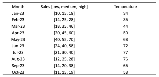
In most cases, the Pandas data frame structure can handle time series data effectively. For univariate time series, a Pandas series with a time index will work just fine. For multivariate time series, a 2-dimensional Pandas data frame with multiple columns will work well. But how about a time series with probabilistic forecasts that have multiple values in each period? Figure (A) shows a multivariate case with the sales and temperature variables. The sales forecasts for each period have low, medium, and high possible values. Although Pandas may still be able to store this dataset, there are special data formats designed to handle complex cases with multiple covariates, multiple periods, and each period with multiple samples.

A good understanding of the data formats will increase your productivity in time series modeling projects. This is the goal of the chapter. We will cover the data formats of the DarTS, GluonTS, Sktime, pmdarima, and Prophet/NeuralProphet libraries. Because Sktime, pmdarima, and Prophet/NeuralProphet are all pandas-compatible, we just need to spend more time on

DarTS
GluonTS

Because the Pandas data frame is the common ground for most data scientists, an easy way to learn is to convert a Pandas data frame to those data formats, and then convert those data formats back to Pandas. In this chapter, we will also explain long-form and wide-form data, and how to covert them between libraries.

Software requirement

Please pip install the following libraries:

!pip install pandas numpy matplotlib darts gluonts sktime pmdarima neuralprophet

Let’s load a long-form dataset.

Get a long-form dataset

We will use the Walmart dataset on Kaggle.com in this chapter. This dataset stacks the multivariate time series data of 45 stores. This dataset was chosen because it is a long-form dataset. A long-form data structure means the data of all groups are stacked vertically. This dataset is loaded as a Pandas data frame.

data = pd.read_csv(path + '/walmart.csv', delimiter=",")
data['ds'] = pd.to_datetime(data['Date'], format='%d-%m-%Y')
data.index = data['ds']
data = data.drop('Date', axis=1)
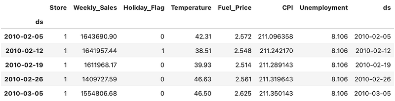
data.head()

The above code converts the string column “Date” to datetime format in Pandas. This step is essential because other libraries often require the date field to be a Pandas datatime format. Figure (B) shows the first few records.

This dataset contains

Date — the week of sales
Store — the store number
Weekly sales — sales for a store
Holiday flag — whether the week is a special holiday week 1 — Holiday week 0 — Non-holiday week
Temperature — Temperature on the day of sale
Fuel price — Cost of fuel in the region

And two macroeconomic indicators that can affect retail sales: the consumer price index, and the unemployment rate. The Walmart dataset stacks the multiple series of 45 stores vertically. Each store has 143 weeks of data.

Make the dataset to be a wide-form

A wide-form data structure means the multivariate time series data of groups are appended horizontally according to the same time index. Below let’s pivot the weekly store sales by store and time.

# pivot the data into the correct shape
storewide = data.pivot(index='ds', columns='Store', values='Weekly_Sales')
storewide = storewide.loc[:,1:10] # Plot only Store 1 - 10
# plot the pivoted dataframe
storewide.plot(figsize=(12, 4))
plt.legend(loc='upper left')
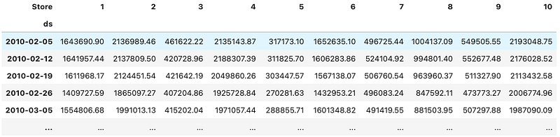
plt.title("Walmart Weekly Sales of Store 1 - 10")

Figure (C) shows the first 10 stores:

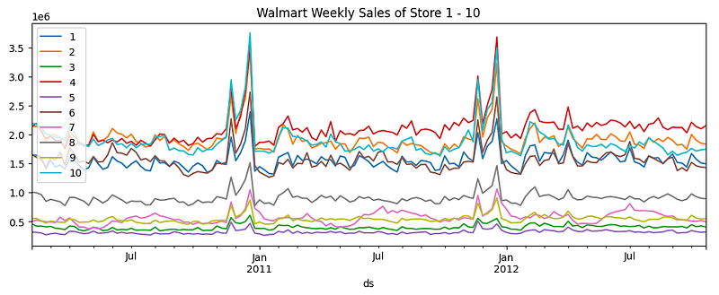
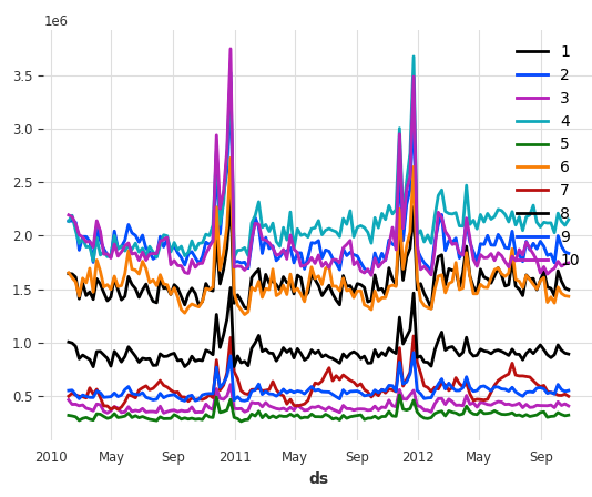
The weekly sales of the 10 stores look like Figure (D):

Figure (D): The plots of the store sales

Let’s inspect the time index. It is a Pandas DateTimeIndex.

print(storewide.index)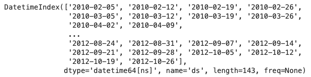

Besides the weekly store sales, you can do the same conversion from long-form to wide-form for any other columns. Now let’s see how the Darts library handles long-form and wide-form datasets.

Darts

The catchy name “Darts” for the Python time series library likely stems from the metaphorical idea of dart throwing, which can represent the process of making accurate predictions or hitting specific targets in data analysis. The darts library aims to provide a unified interface for working with various time series forecasting models including univariate and multivariate time series. It is widely used by time series data scientists.

The main data class of darts is its “TimeSeries” class. Darts store the values in an array of shapes (time, dimensions, samples):

Time: The time index, like the 143 weeks in the above example.
Dimensions: The “columns” of multivariate series
Samples: The values of a column and time. In Figure (A), the values for the first period are [10,15,18]. It is not a single value but a list of values. For example, the probabilistic forecasts for a future week can be three values at the 5%, 50%, and 95% quantiles. It is conventionally called “samples”

Darts — from a long-form Pandas data frame

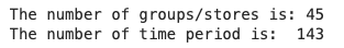
To convert the long-form Walmart data to a darts data format, you just use the from_group_datafrme() function. The function takes two key inputs: group_cols for the group id and time_col for the time index. The group_cols in our case is the “Store” column, and the time_col is the time index “ds”.

from darts import TimeSeries
darts_group_df = TimeSeries.from_group_dataframe(data, group_cols='Store', time_col='ds')
print("The number of groups/stores is:", len(darts_group_df))
print("The number of time period is: ", len(darts_group_df[0]))

Store 1 data are stored in darts_group_df[0], and Store 2 in darts_group_df[1], and so on. There are 45 stores, so the length of the darts data darts_group_df is 45. Each store has 143 weeks, so the length of Store 1, darts_group_df[0], is 143.

Let’s see what the data look like:

darts_group_df

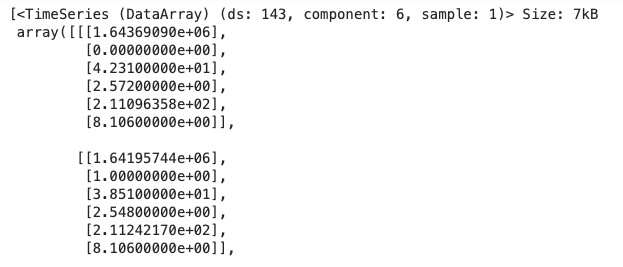
Figure (E): The darts data format for the Walmart store sales data

Figure (E) states (ds: 143, component:6, sample:1) for 143 weeks, 6 columns, and 1 sample for each store and week. The data for Store 1 is darts_group_df[0]. You can list the column names by using the .components function.

darts_group_df[0].components

The column names are:

Index([‘Weekly_Sales’, ‘Holiday_Flag’, ‘Temperature’, ‘Fuel_Price’, ‘CPI’, ‘Unemployment’], dtype=’object’, name=’component’)

Now let’s continue to learn how to convert a wide-form data frame to the darts data structure.

Darts — From a wide-form Panda data frame

You just use the.from_dataframe() function of the TimeSeries class in Darts:

from darts import TimeSeries
darts_df = TimeSeries.from_dataframe(storewide)
darts_df

The outputs are shown in Figure (F):

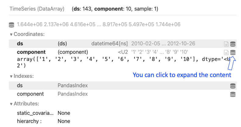
Figure (F): Darts DataArray (image by author)

Figure (F) states (ds: 143, component:10, sample:1) for 143 weeks, 10 columns, and 1 sample for each store and week. You can expand the small icon to see the component, which refers to the column names.

Now let’s learn how to plot with Darts.

Darts — plotting

The plotting syntax is as easy as the one in Pandas. You simply do .plot():

darts_df.plot()

Figure (D) shows the plot:

What if we have a single series? Let’s learn how to convert to Darts.

Darts — from a univariate Pandas series

The column storewide[1] is a Pandas series for Store 1. You can use .from_series() to convert a Pandas series to Darts conveniently:

darts_str1 = TimeSeries.from_series(storewide[1])
darts_str1

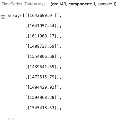
Figure (E) shows the output. It has 143 weeks, 1 column, and 1 sample in each week, as shown in (ds:143, component:1, sample:1).

Figure (E): The data structure of a series

And plotting is the same as shown in Figure (F):

darts_str1.plot()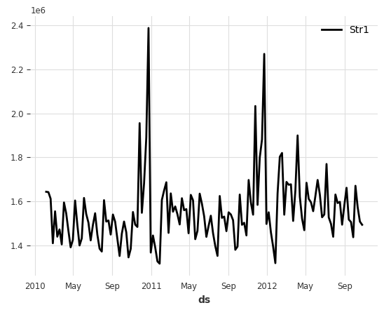

Great. Now let’s learn how to convert a Darts dataset back to a Pandas data frame.

Darts — converting back to pandas

You simply use .pd_dataframe():

# Convert a darts dataframe to pandas dataframe
darts_to_pd = TimeSeries.pd_dataframe(darts_df)
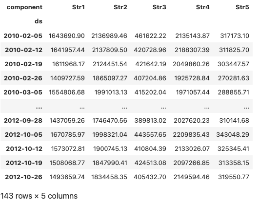
darts_to_pd

The output is a 2-dimensional Pandas data frame:

Not all Darts data can be converted to a 2-dimensional Pandas data frame. For example, if there are multiple values like probabilistic forecasts for a store of a week, we can not store the data in a 2-D Pandas data frame. In such a case, we can output the data to Numpy arrays.

Darts — converting to Numpy array

Darts lets you use .all_values to output all values in arrays. The drawback is the time index is dropped.

# Export all series to numpy array containing the values of all series.
# https://unit8co.github.io/darts/userguide/timeseries.html#exporting-data-from-a-timeseries
TimeSeries.all_values(darts_df)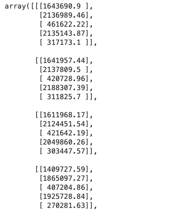

Having learned the data structure of Darts, let’s learn the data structure of another popular time series library — Gluonts.

Gluonts:

Gluonts is a Python library developed by Amazon to handle time series data. The Gluonts library includes many modeling algorithms, especially neural network-based. These models can handle univariate and multivariate series and probabilistic forecasts. A Gluonts dataset is a list of time series in Python dictionary format. Let’s see how to convert a long-form Pandas data frame to Gluonts.

Gluonts — From a long-form Pandas data frame

The gluons.dataset.pandas class has many convenient functions for handling Pandas data frames. To load a long-form dataset in Pandas, you simply use .from_long_dataframe():

# Method 1: from a long-form
from gluonts.dataset.pandas import PandasDataset
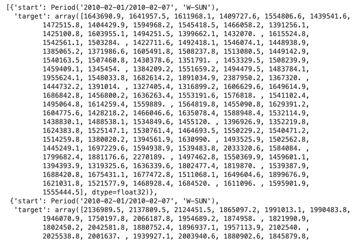
data_long_gluonts = PandasDataset.from_long_dataframe(data, target="Weekly_Sales", item_id="Store", timestamp='ds', freq='W')
data_long_gluonts

When you print the Gluonts dataset, it shows the metadata:

PandasDataset<size=45, freq=W, num_feat_dynamic_real=0, num_past_feat_dynamic_real=0, num_feat_static_real=0, num_feat_static_cat=0, static_cardinalities=[]>

Now let’s learn how to load from a wide-form.

Gluonts — From a wide-form Pandas data frame

The PandasDataset() class expects a dictionary of time series. So you will first convert the wide-form Pandas data frame into a Python dictionary, then use PandasDataset():

# Method 2: from a wide-form
from gluonts.dataset.pandas import PandasDataset
data_wide_gluonts = PandasDataset(dict(storewide))
data_wide_gluonts

Often we split a Pandas data frame into the training (“in-time”) and test (“out-of-time”) data like below.

len_train = int(storewide.shape[0] * 0.85)
len_test =  storewide.shape[0] - len_train 
train_data = storewide[0:len_train]
test_data = storewide[len_train:]
[train_data.shape, test_data.shape] # The output is [(121,5), (22,5)

As said before, a Gluonts dataset is a list of data in the Python dictionary format. We always can use the ListDataset() class in Gluonts. Let’s convert the data using ListDataset():

Gluonts — ListDataset() for any general conversion

A Gluonts dataset is a list of time series in Python dictionary format you can use ListDataset() as the general conversion tool. The ListDataset() class expects the basic elements of a time series such as the starting time, the value, and the frequency of the period.

Let’s convert the wide-form store sales in Figure (C). Each column in the data frame is a Pandas series with a time index. Each Pandas series will be converted to the Pandas dictionary format. The dictionary shall have two keys: FieldName.START and FieldName.TARGET. The Gluonts dataset therefore is a list of time series in Python dictionary format.

def convert_to_gluonts_format(dataframe, freq):
    start_index = dataframe.index.min()
    data = [{
                FieldName.START:  start_index,
                FieldName.TARGET:  dataframe[c].values,
            }
            for c in dataframe.columns]
    #print(data[0])
    return ListDataset(data, freq=freq)
train_data_lds = convert_to_gluonts_format(train_data, 'W')
test_data_lds = convert_to_gluonts_format(test_data, 'W')
train_data_lds

The outcome is a list of Python dictionaries. Each dictionary has the key start for the time index and the key target for the value:

Next, let’s learn how to convert a Gluonts dataset back to a Pandas data frame.

Gluonts — converting back to Pandas

A Gluonts dataset is a list of Python dictionaries. To convert a Gluonts dataset back to a Python data frame, first, you will make the Gluonts dictionary data iterable. You will enumerate the keys in the Gluonts dataset and use a for-loop to output.

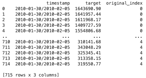
In our Walmart store sales data, there are three keys: the timestamps, the weekly sales, and the store ID. So we create three columns in the output data frame: timestamps, target_values, and index.

# Convert a gluonts dataset to a pandas dataframe
# Either long-form or wide-form

the_gluonts_data = data_wide_gluonts # you can also test data_long_gluonts

timestamps = [] # This is the time index
target_values = [] # This is the weekly sales
index = [] # this is the store in our Walmart case

# Iterate through the GluonTS dataset
for i, entry in enumerate(the_gluonts_data):
    timestamp = entry["start"]
    targets = entry["target"]
    
    # Append timestamp and target values for each observation
    for j, target in enumerate(targets):
        timestamps.append(timestamp)
        target_values.append(target)
        index.append(i)  # Keep track of the original index for each observation

# Create a pandas DataFrame
df = pd.DataFrame({
    "timestamp": timestamps,
    "target": target_values,
    "original_index": index
})

print(df)

The above code stacks the data of all stores vertically to output a long-form Pandas data frame.

This book gives more examples of Gluonts. You can go to the following chapters to learn how to model with Gluonts:

Furthermore, the complex data structure of Darts and Gluonts supports modeling algorithms that can build global models of multiple time series and probabilistic forecasts. A global model refers to a single model for multiple time series. It is widely used when there is a consistent underlying pattern or relationship across all the time series. The time series data in our Walmart case is an ideal case for a global model. In contrast, if a separate model is fitted to each of the multiple time series, the model is called a local model. In the Walmart data, we shall build 45 local models because there are 45 stores.

After learning the data structure of Darts and Gluonts. We will continue to learn the data formats of Sktime, pmdarima, and Prophet/NeuralProphet. As said earlier, the data formats of the three libraries are pandas-compatible. So there is no data conversion. This makes our learning much easier.

Sktime

Sktime is designed to integrate with scikit-learn to leverage a wide range of scikit-learn time series algorithms. It aims to simplify the process of working with time series data by providing a unified interface and implementation of common time series analysis tasks. It provides a wide range of tools for handling and analyzing time series data, including algorithms for forecasting, classification, clustering, and more. Below is an example from A Tutorial on Multi-period Time Series Forecasts:

import lightgbm as lgb
from sktime.forecasting.compose import make_reduction

lgb_regressor = lgb.LGBMRegressor(num_leaves = 10,
              learning_rate = 0.02,
              feature_fraction = 0.8,
              max_depth = 5,
              verbose = 0,
              num_boost_round = 15000,
              nthread = -1
)
lgb_forecaster = make_reduction(lgb_regressor, window_length=30, strategy="recursive")
lgb_forecaster.fit(train)

You are encouraged to read the chapter A Tutorial on Multi-period Time Series Forecasts. to learn more about Sktime. Next, let’s learn pmdarima.

Pmdarima

Pmdarima is a Python wrapper for ARIMA and SARIMA models, building upon the popular statsmodels library. It automatically selects the optimal ARIMA model with great functionality and convenience. The data should be a one-dimensional array or pandas Series. Below is an example from Automatic ARIMA, where the data frame “train” is a Pandas data frame.

import pmdarima as pm
model = pm.auto_arima(train,
                      d=None,
                      seasonal=False,
                      stepwise=True,
                      suppress_warnings=True,
                      error_action="ignore",
                      max_p=None,
                      max_order=None,
                      trace=True)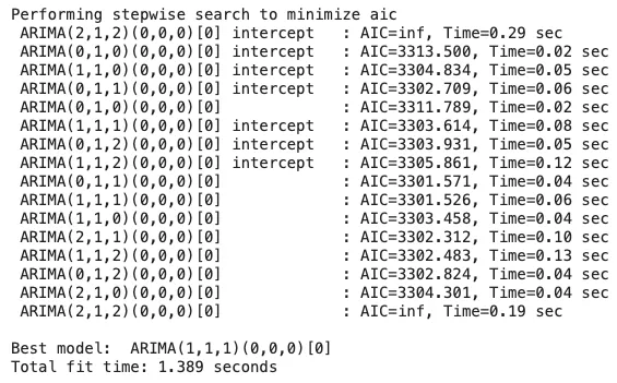

From here you can go to the following chapter to learn how to model with pmdarima:

Automatic ARIMA!

Prophet/NeuralProphet

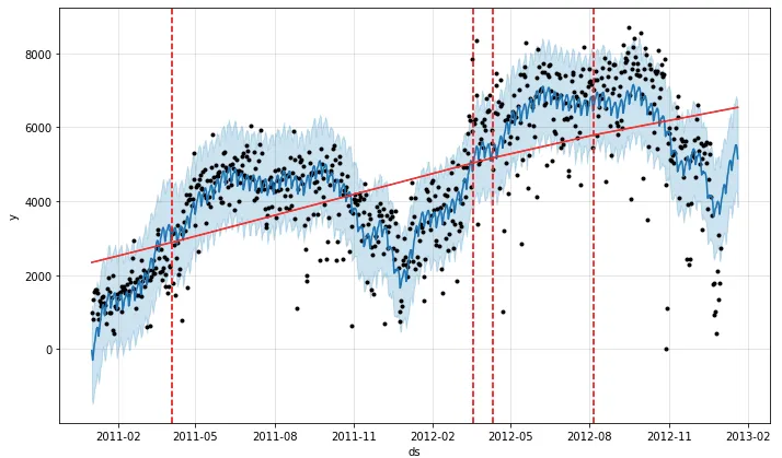
Prophet is a time series forecasting library developed by Facebook. It automatically detects seasonal patterns, handles missing data, and incorporates holiday effects into its forecasting models. If you have used the Prophet library, you will like its user-friendly interface and interactive plotly-style outputs. Prophet enables analysts to generate forecasts with minimal manual intervention. Prophet has become popular for its flexible trend modeling capabilities and built-in uncertainty estimation.

Prophet performs univariate time series modeling. It expects a Pandas data frame with column names [‘ds’,’y’]. Below is an example in Business Forecasting with Facebook’s “Prophet” that loads a Pandas data frame “bike” to train a Prophet model.

import pandas as pd
from prophet import Prophet
bike.columns = ['ds','y']
m = Prophet()
m.fit(bike)

Prophet’s plot is appealing, making it a versatile choice for analysts.

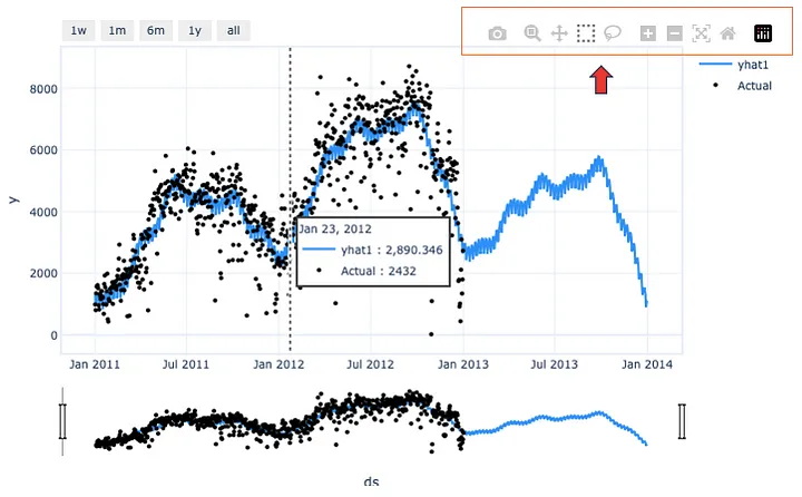
Building on the framework of Prophet, NeuralProphet has significantly enhanced Prophet’s additive model with a neural network architecture. It allows for more flexible and complex modeling of time series data. It integrates the strengths of Prophet, such as automatic seasonality detection and holiday effects handling. NeuralProhet also focuses on univariate time series forecasting. Below is an example from the previous chapter Tutorial I: Trend + seasonality + holidays & events that loads a Pandas data frame to train a NeuralProphet model.

from neuralprophet import NeuralProphet
df = pd.read_csv(path + '/bike_sharing_daily.csv')

# Create a NeuralProphet model with default parameters
m = NeuralProphet()
# Fit the model
metrics = m.fit(df)

It plotting capacity is appealing like Prophet.

From here you can go to the following chapters to learn how to model with Prophet/NeuralProphet:

Conclusions

This chapter surveyed the five Python time series libraries used in this book. We have learned the data structures of the Darts and the Gluonts libraries. We learned how to convert a pandas data frame to each library and convert it back to pandas. We surveyed Sktime, pmdarima, and Prophet/NeuralProphet libraries as well. It is important to keep in mind that all these libraries have their relative strengths and features. The choice of a Python library depends on your requirement for speed, integration with other Python environments, and model proficiency. This chapter can increase your productivity in building time series models in the next few chapters.