Quantile Regression for Time Series Probabilistic Forecasts

We often hear “the only thing that is certain is that nothing is certain.” We do not like uncertainty. We do not want to hear “tomorrow’s weather is 50% heatwave and 50% hurricane.” But ironically we also ask for forecasting data to come with uncertainty. We still want certainty in uncertainty to help us plan for future. Assume we are doing the financial planning for an organization, which one of the two will be better:

The expected average financial loss is $40M, or
We have 95% confidence that the financial loss will be between $10M and $70M, with an average of around $40M. Further, we have 68% confidence that the financial loss will be between $30M and $50M.

Quantile regression meets this need. It provides the prediction intervals with quantified chances as shown in Figure (A). Quantile regression is a statistical technique used for modeling the relationship between predictor variables and a response variable, particularly when the conditional distribution of the response variable is of interest. Unlike traditional regression methods that focus on estimating the conditional mean of the response variable given the predictors (e.g., ordinary least squares regression), quantile regression estimates the conditional quantiles of the response variable.

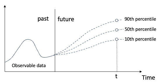
We learned the Monte Carlo simulation technique in “Monte Carlo Simulation for Time Series Probabilistic Forecasts”. What are the advantages of quantile regression over Monte Carlo simulation? First, Quantile regression directly estimates the conditional quantiles of the response variable given the predictors. This means that instead of generating a large number of possible outcomes as in Monte Carlo simulation, quantile regression provides estimates of specific quantiles of the response variable’s distribution. This can be particularly useful for understanding prediction uncertainty at different levels, such as the median, quartiles, or extreme quantiles. Second, quantile regression provides a model-based approach to estimating prediction uncertainty. It utilizes the observed data to estimate the relationship between variables and makes predictions based on this relationship. In contrast, Monte Carlo simulation relies on specifying probability distributions for input variables and generating outcomes based on random sampling.

We have learned how to build time series models with NeuralProphet in

Neural Prophet provides two statistical techniques: (1) quantile regression and (2) conformal quantile prediction. The conformal quantile prediction technique adds a calibration process to quantify regression. In this chapter, we will perform the quantile regression module of Neural Prophet. We will learn conformal quantile prediction in next chapter. The Python notebook is available via this Github link for download.

Software requirement

You will follow the standard installation pip install NeuralProphet to install NeuralProphet.

!pip install neuralprophet

If you use Google Colab, just be aware that NeuralProphet does not work with Colab unless using numpy1.23.5. You will need to uninstall numpy and install numpy1.23.5.

# neuralprophet does not work with colab unless numpy1.23.5: https://github.com/googlecolab/colabtools/issues/3752
!pip uninstall numpy
!pip install git+https://github.com/ourownstory/neural_prophet.git numpy==1.23.5

And let’s import several tools:

%matplotlib inline
from matplotlib import pyplot as plt
import pandas as pd
import numpy as np
import logging
import warnings
logging.getLogger('prophet').setLevel(logging.ERROR)
warnings.filterwarnings("ignore")

Continuing with the previous chapters on NeuralProphet, I will the Bike Share Daily data from Kaggle (here or here). This dataset is a multivariate dataset that has the daily rental demand, and other weather fields like temperature or wind speed.

from google.colab import drive
drive.mount('/content/gdrive')
path = '/content/gdrive/My Drive/data/time_series'
data = pd.read_csv(path + '/bike_sharing_daily.csv')
data.tail()

Let’s plot the bike-sharing count. We observe the demand increases in the second year, and there is a seasonal pattern.

# convert string to datetime64
data["ds"] = pd.to_datetime(data["dteday"])

# create line plot of sales data
plt.plot(data['ds'], data["cnt"])
plt.xlabel("date")
plt.ylabel("Count")
plt.show()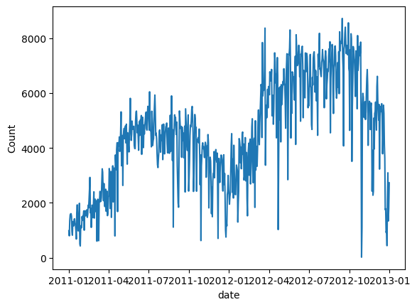

Figure (C): The bike-rental daily demand

We will do a very minimal data preparation for modeling. NeuralProphet requires the column names to be “ds” and “y” which is the same as Prophet.

df = data[['ds','cnt']]
df.columns = ['ds','y']

Let’s go on directly to build the quantile regression in NeuralProphet. Assume we want the values for the 5th, 10th, 50th, 90th, and 95th quantile. We specify quantile_list = [0.05,0.1,0.5,0.9,0.95] and turn on the quantile “parameter quantiles = quantile_list”. The rest parameters are the same as those in Chapter 3: Tutorial I: Trend + seasonality + holidays & events.

from neuralprophet import NeuralProphet, set_log_level

quantile_list=[0.05,0.1,0.5,0.9,0.95 ]
# Model and prediction
m = NeuralProphet(
    quantiles=quantile_list,
    yearly_seasonality=True,
    weekly_seasonality=True,
    daily_seasonality=False
)
m = m.add_country_holidays("US")
m.set_plotting_backend("matplotlib")  # Use matplotlib

df_train, df_test = m.split_df(df, valid_p=0.2)
metrics = m.fit(df_train, validation_df=df_test, progress="bar")
metrics.tail()

Once done, we will make a new data frame for the forecasts by using .make_future_dataframe(). NeuralProphet inherits this from Prophet. The parameter n_historic_predictions is set to 100 to include only the past 100 data points. If it is set to “True”, it will include the entire history. We set “periods=50” to forecast the next 50 data points.

future = m.make_future_dataframe(df, periods=50, n_historic_predictions=100) #, n_historic_predictions=1)

# Perform prediction with the trained models
forecast = m.predict(df=future)
forecast.tail(60)

The forecasts are stored in the data frame “forecast”.

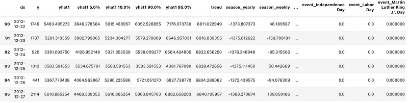
The above data frame has all the data elements for plotting.

m.plot(
    forecast, 
    plotting_backend="plotly-static"
    #plotting_backend = "matplotlib"
)

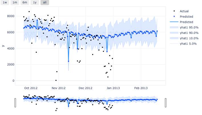
The plot looks like below. Notice the prediction intervals are provided by the quantile values!

Prediction intervals and confidence intervals are different

As prediction intervals become popular, it will be helpful to distinguish the difference between prediction intervals and confidence intervals. Both statistical concepts are used to quantify uncertainty, but they have different objective, calculation, and applications. Since most people learned confidence intervals in the regression unit of a statistics course, I will use a regression to explain the differences. In Figure (F) I draw a linear regression in the left and the quantile regressions in the right.

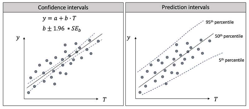
Figure (F): The differences between confidence intervals and prediction intervals

First, their objectives are different:

Linear regression: its primary goal is to find the line such that the predicted values are as close as possible to the conditional mean of the dependent variable for a given value of the independent variable.
Quantile regression: Its goal is to provides a range of values within which future observations are expected to fall, given a certain level of confidence. It estimates the relationship between the independent variables (in our case, T) at different quantiles of the conditional distribution of the dependent variable Y.

Second, their calculations are different:

In linear regression, a confidence interval is an interval estimate for the coefficients of the independent variables, like b ± 1.96 * standard error of b in Figure (F). It typically uses ordinary least squares (OLS) to find the minimum total distance from the data points to the line. Because the coefficients can vary, the predicted conditional mean, Y, can vary.
In quantile regression, you will select a quantile level such as 25th, 50th, or 75th quantile, of the depedent variable to estimate the regression coefficients. Quantile regression typically minimizes a weighted sum of absolute deviations but not OLS.

Third, their applications are different:

In linear regression, you will say “the predicted conditional mean is such and such with 95% confidence interval. Confidence intervals are narrower than the prediction intervals because they are the conditional mean but not the entire range.
In quantile regression, you will say “there is a 95% chance that the predicted values fall in the range of the prediction intervals.

Conclusions

In this chapter we learned the concept of quantile regression for prediction intervals. We demonstrated how to generate prediction intervals with NeuralProphet. We have also distinguish the differences between prediction intervals and confidence intervals, a common confusion in business applications. Next chapter we will continue to study another important techniques for prediction uncertainty — the conformal quantile regression (CQR).