Automatic ARIMA!

Automatic model selection and multi-step forecasting

ARIMA (AutoRegressive Integrated Moving Average) is a statistical model used for time series forecasting and analysis. The origin of ARIMA can be traced back to the early 1900s with the development of autoregressive (AR) models and moving average (MA) models separately. Neither model appears sufficient to capture the complex dynamics of real-world time series data. In the 1960s, the AR and MA models were formally united into ARIMA by three statisticians: George E. P. Box, Gwilym M. Jenkins, and Gregory C. Reinsel in their book “Time Series Analysis: Forecasting and Control.”

Since ARIMA probably is the well-known paradigm, why do I still include it in this “modern” time series book? The primary reason is that AR and MA leave many footprints in many modern time series techniques. A comprehensive understanding of ARIMA helps us to leverage to other complex models. For example, we have seen the AR module in NeuralProphet, “Tutorial II: Trend + seasonality + holidays & events + auto-regressive (AR) + lagged regressors + future regressors.” And we will see the AR terms as the features in supervised-learning models in “A Tutorial on Tree-based Time Series Forecasting” and “A Tutorial on Multi-step Time Series Forecasts.” We do see the work of AR and MA in modern time series techniques.

Today’s code libraries have automated the search for optimal ARIMA models to some degree. If you were trained by the standard ARIMA school, you may have memorized its stylized instruction for the selection of the optimal orders of AR and MA. You are to use the Auto-correlation Function (ACF) and the partial Auto-correlation Function (PACF) to determine the model specifications. However, I tend to forget those stylized instructions but just build many candidate models of various orders to select the optimal model. Why don’t we generate many models to select the best model? For this reason, there are handy libraries such as “pmdarima” in Python to automate the search for optimal specifications. I title this chapter as the Automatic ARIMA to emphasize this advantage. Still, I will cover the concepts of Differencing, ACF, and PACF.

Modern code libraries like the “statsmodels” and “pmdarima” libraries can produce multi-step forecasts instead of the one-period-ahead forecast. They do so by applying the model recursively to produce forecasts. In this chapter, we will learn how to do it. Generally speaking, multi-step forecasting strategies can apply to many other types of models not just ARIMA. In “A Tutorial on Multi-step Time Series Forecasts,” I explain the leap from one-period-ahead to multi-period-ahead, and how the strategies enable other modeling techniques.

Finally, in many use cases, we are not satisfied with a point estimate but need the prediction intervals. We need the range of possible values to evaluate the potential uncertainties. The “pmdarima” and “statsmodels” libraries also provide the prediction intervals. I will showcase the prediction intervals as well. I would like to point out that the prediction interval technique in “pmdarima” and “statsmodels” is a simple prediction interval that has a fixed length for all periods, in contrast to the advanced prediction intervals like conformalized quantile regression (Romano, Y., Patterson, E., & Candès, E.J. (2019)) that have varying interval length. The varying interval length has its practical applications and I will illustrate in a later chapter.

In this post, I will explain the theory and practice comprehensively. I will use real-world data to walk you through the model building and forecasting. Feel free to skim through a section you are already familiar with. The Python notebook is here for download. The topics are:

The ARIMA models
Differencing
Use the ACF to suggest the orders of MA
Use the PACF to suggest the orders of AR
The use of the pmdarima library to search for the optimal model automatically
The multi-step forecasts
The use of statsmodels to update the model in iterations
The SARIMA models

Let’s load the data first.

Data pre-processing

We will use the avocado sales from Kaggle.

%matplotlib inline
from matplotlib import pyplot as plt
import pandas as pd
import numpy as np

from google.colab import drive
drive.mount('/content/gdrive')

path = '/content/gdrive/My Drive/data/time_series'
data = pd.read_csv(path + '/avocado_monthly.csv', index_col='Date')
data.sort_values(by='Total Volume', ascending=False)

This dataset has monthly time series for several regions and types.

We will just use one univariate time series from this dataset.

# Take only one time series, which is type = 'organic' and region = 'TotalUS'
df = data[(data['type']=='organic') & (data['region']=='TotalUS')].copy()
df = df['Total Volume']
df.columns = ['y']
df = df[pd.to_datetime(df.index)<=pd.to_datetime('2018-02-01')]

# Plot the univariate time series
plt.figure(figsize=(10,4))
plt.plot(df)
plt.xlabel("Date")
plt.ylabel("Volume")
plt.show()

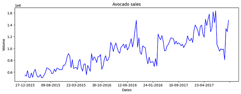
The time series looks like this:

Then we use 80% as the in-time training data and the rest 20% as the out-of-time test data.

# Train-test-split
train_len = int(df.shape[0] * 0.8)
train, test = df[:train_len], df[train_len:]
print(f"{train_len} train samples")
print(f"{df.shape[0] - train_len} test samples")

Good. Now we start with the definitions.

The ARIMA models

ARIMA is a class of models that fit a univariate time series to forecast future values. The models use the past or the lagged values of the time series, namely the auto-regressive (AR) terms, and the lagged forecast errors, the moving average (MA) terms, to forecast the future values. The term ARIMA is the acronym for “Auto-Regressive-Integrated-Moving-Average.” It is composed of “AR”, “I”, and “MA”. The “I” in ARIMA stands for “integrated,” which means that the time series has been differenced to achieve stationarity. A stationary time series has constant mean, variance, and autocorrelation over time, making it easier to model. The model is called an ARIMA(p,d,q) model that is completely described by three parameters — p, d, and q:

p is the order of the AR term
q is the order of the MA term
d is the number of differencing required to make the time series stationary

In mathematical form, it is:

Let’s get familiar with the ARIMA notations by apply the about equation.

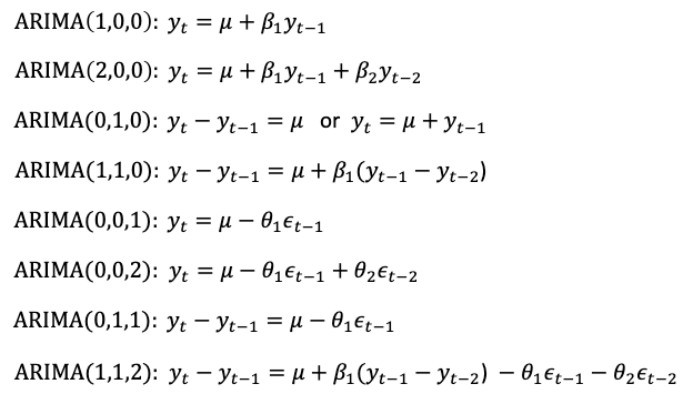
Typically we see AR only or MA only, or p and q together are less than 4 so there are not many terms on the right-hand side.

Differencing

The goal of differencing is to make the time series stationary. In a time series, stationarity means the average of the values remains constant over time. In other words, a stationary time series has a constant mean. Below let me plot the original time series of the training data, its 1st differencing (differencing once) and 2nd differencing (differencing twice).

import numpy as np, pandas as pd
from statsmodels.graphics.tsaplots import plot_acf, plot_pacf
from statsmodels.tsa.stattools import adfuller
import matplotlib.pyplot as plt
plt.rcParams.update({'figure.figsize':(10,6), 'figure.dpi':100})
lag_len = 15
fig, axes = plt.subplots(3, 1, sharex=True)

# Original Series
axes[0].plot(train.values); axes[0].set_title('Original Series')

# 1st Differencing
axes[1].plot(train.diff()); axes[1].set_title('1st Order Differencing')


# 2nd Differencing
axes[2].plot(train.diff().diff()); axes[2].set_title('2nd Order Differencing')

axes[0].xaxis.set_major_locator(MultipleLocator(30))

plt.show()

The outputs are:

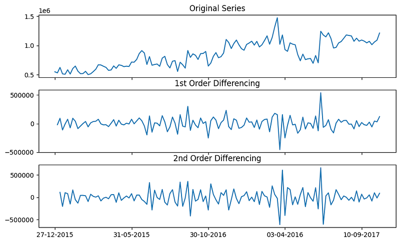
You can see the 1st and 2nd differenced time series are stationary. This means the model should be differenced at least once. Typically the 1st differencing is enough. Differencing for a stationary time series still will be stationary. If the 1st differencing is already stationary, you do not need to over-difference to get the 2nd differencing.

Now let’s understand how to use the ACF to get the orders of MA.

Use the ACF to suggest the orders of MA

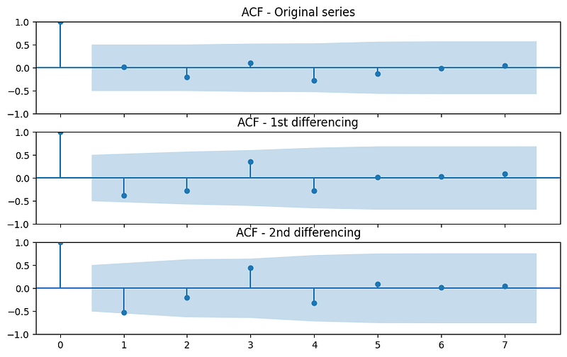
You are already familiar with the correlation coefficient between two variables. It measures how they are related. It takes values between -1 and 1. A correlation coefficient of -1 indicates a perfect negative linear relationship, meaning that as one variable increases, the other variable decreases. A correlation coefficient of 1 indicates a perfect positive linear relationship, meaning that as one variable increases, the other variable also increases. A correlation coefficient of 0 indicates no linear relationship between the variables. Similarly, the autocorrelation of y at lag k is the correlation between y and itself lagged by k periods, i.e., it is the correlation between yt and yt-k. Below let’s plot the autocorrelations.

from statsmodels.graphics.tsaplots import plot_acf
plt.rcParams.update({'figure.figsize':(10,6), 'figure.dpi':100})
lag_len = 15
fig, axes = plt.subplots(3, 1, sharex=True)

# Original Series
plot_acf(train.values[0:lag_len], ax=axes[0], title = 'ACF - Original series')

# 1st Differencing
plot_acf(train.diff().dropna()[0:lag_len], ax=axes[1], title = 'ACF - 1st differencing')

# 2nd Differencing
plot_acf(train.diff().diff().dropna()[0:lag_len], ax=axes[2], title = 'ACF - 2nd differencing')

plt.show()

The correlation coefficients are shown below. The correlation coefficient of the first bar is 1.0 because it is the correlation of y_t with itself. The blue region is the significance limit. A bar crossing the significance limit means it is statistically significant. As you can see, lag 1 in the 1st differencing line is significant. This means the model is expected to have the lag 1 term and there is the 1st differencing.

Now let’s learn PACF.

Use the PACF to suggest the orders of AR

ACF measures the correlation between a time series and its lagged values. It tells us how much the current value of the time series is related to its past values. PACF, on the other hand, measures the partial correlation between a time series and its lagged values, after accounting for the effects of all the lagged values that come before it. It helps us determine whether there is a direct relationship between the current value of the time series and a specific lagged value, after controlling for the effects of all the other lagged values. You can observe that PACF lag 1 is quite significant since it is well above the significance line. Lag 2 turns out to be significant as well, slightly managing to cross the significance limit (blue region).

from statsmodels.graphics.tsaplots import plot_pacf
plt.rcParams.update({'figure.figsize':(10,6), 'figure.dpi':100})
lag_len = 15
fig, axes = plt.subplots(3, 1, sharex=True)

# Original Series
plot_pacf(train.values[0:lag_len], ax=axes[0], title = 'PACF - Original series')

# 1st Differencing
plot_pacf(train.diff().dropna()[0:lag_len], ax=axes[1], title = 'PACF - 1st differencing')

# 2nd Differencing
plot_pacf(train.diff().diff().dropna()[0:lag_len], ax=axes[2], title = 'PACF - 2nd differencing')

plt.show()

The outputs are:

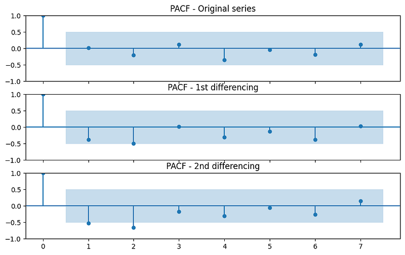
The above differencing, ACF, and PACF suggest ARIMA(1, 1, 1). Suppose we do not know the above diagnosis, we still can use auto_ARIMA() to search for a range of model specifications.

The use of auto_ARIMA() to search for the optimal model automatically

import pmdarima as pm
model = pm.auto_arima(train,
                      d=None,
                      seasonal=False,
                      stepwise=True,
                      suppress_warnings=True,
                      error_action="ignore",
                      max_p=None,
                      max_order=None,
                      trace=True)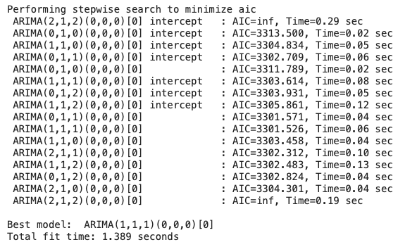

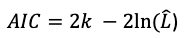
The Akaike Information Criterion (AIC) value is a model performance metric. It is 2 * the number of model parameters minus 2 times the maximum likelihood (L). A smaller value indicates a better-fitted model.

The lowest AIC value is 3,301.526 of ARIMA(1,1,1), so it is concluded to be the best model. We have turned off the seasonal hyper-parameter, so the seasonal orders are (0,0,0). Next, let’s produce the forecasts.

The multi-step forecasts

When you fit an ARIMA model using pmdarima, it internally leverages the “predict” function in “statsmodels” to generate forecasts. The “predict” function allows you to specify the number of periods for the future horizon. Below we set the future horizon to the length of the test data. And we set “return_conf_int = True” and “alpha = 0.05” to return the confidence intervals at the 95% confidence level.

# Create multi-step forecasts for the length of test_len
fcast = model.predict(n_periods=test_len, return_conf_int=True, alpha=0.05)
forecasts = fcast[0]
confidence_intervals = fcast[1]

Let’s plot the training and the test data, the predictions, and the confidence intervals.

def plot_it():
    fig, ax = plt.subplots(figsize=(12,4))

    # Actual vs. Predicted
    ax.plot(train, color='blue', label='Training data')
    ax.plot(test.index, forecasts, color='red', marker='o',
                label='Predicted')
    ax.plot(test.index, test, color='green', label='Test data')
    ax.set_title('Avocado sales')
    ax.set_xlabel('Dates')
    ax.set_ylabel('Volume')
    conf_int = np.asarray(confidence_intervals)

    # Confidence intervals
    ax.fill_between(test.index,
                        conf_int[:, 0], conf_int[:, 1],
                        alpha=0.9, color='orange',
                        label="Confidence Intervals")
    # Make a plot with major ticks that are multiples of 20
    ax.legend()
    ax.xaxis.set_major_locator(MultipleLocator(20))
    plt.show()

plot_it()

The plot is:

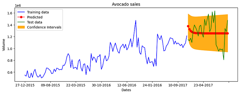
The outcome is a straight line and does not look impressive. Why? It is because we use small and simple data. We can improve it by updating the model in each iteration. Before we do that, let’s evaluate the model performance.

from sklearn.metrics import mean_squared_error, mean_absolute_percentage_error
print(f"MAPE: {mean_absolute_percentage_error(test, forecasts)}")

The mean absolute percentage error is 0.1490595592393948 or 14.9%. Let’s keep this value in mind. We will compare it with later experiments.

Update the model in each iteration

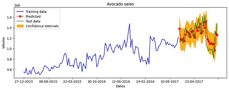
Even prediction adds a new observation to the forecasting horizon. If the model is static, the predictions become a straight line as the above. But according to the statsmodels function documentation, we actually can update the model with the added observation in every iteration.

Below we will forecast only one period in each iteration of the out-of-time test period. We append the new prediction and update the model. The code below also requests the confidence intervals by using “return_conf_int = True” and “alpha= 5%”. It simply adds a prediction interval for each predicted value at the 95% confidence level.

def one_period_forecast():
    fcast = model.predict(n_periods=1, return_conf_int=True, alpha=0.05)
    # fcast is a list of two lists.
    # The first list is the forecast
    forecasts = fcast[0].tolist()
    # The second list is the confidence interval
    confidence_intervals = fcast[1]
    return ( forecasts, 
             np.asarray(confidence_intervals).tolist()[0])

forecasts = []
confidence_intervals = []

for add_obs in test:
    fc, conf = one_period_forecast()
    forecasts.append(fc)
    confidence_intervals.append(conf)
    # Updates the existing model
    model.update(add_obs)

plot_it()

When the model can be updated in each iteration, the fitness appears better.

How about the model performance?

print(f"MAPE: {mean_absolute_percentage_error(test, forecasts)}")

The MAPE is 0.11766234388644323, slightly improved than the above 11.7%.

We have limited the model to ARIMA only. Since it is a multi-year time series, we suspect it possesses strong seasonality. We will relax the model by using Seasonal ARIMA.

The SARIMA models

SARIMA just applies seasonal differencing. Seasonal differencing is similar to regular differencing. Rather than subtracting consecutive terms, seasonal differencing subtracts the value from the previous season. The SARIMA models are generally written as SARIMA(p,d,q)(P,D,Q)[S] where

p is the order of the seasonal AR term
q is the order of the seasonal MA term
Q is the order of seasonal differencing
S is the seasonal cycle such as 12 for 12 months.

The seasonal ARIMA model incorporates additional parameters to capture the seasonal patterns in the data. It adds the following components:

Seasonal AR terms: These terms represent the relationship between the current observation and a certain number of lagged observations at seasonal intervals. It captures the seasonal patterns in the data.
Seasonal MA terms: These terms represent the relationship between the current observation and a certain number of lagged forecast errors at seasonal intervals. It captures the seasonal fluctuations in the data.

It is very easy to do SARIMA modeling. All we need to do is to turn the hyper-parameter “seasonal” to “True”.

import pmdarima as pm
model = pm.auto_arima(train,
                      # You just need to turn the seasonal to "True"
                      seasonal=True,
                      start_P=1,
                      start_q=1,
                      max_p=None,
                      max_q=None,
                      m=12,
                      d=1,
                      D=1,
                      trace=True,
                      error_action='ignore',
                      suppress_warnings=True,
                      stepwise=True)
model.summary()

It has built several candidate models. The best model is ARIMA(0,1,1)(0,1,1)[12].

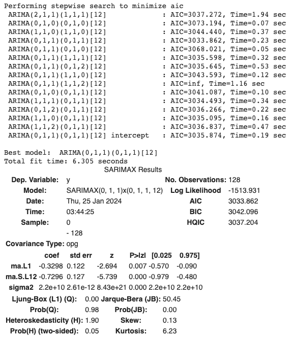
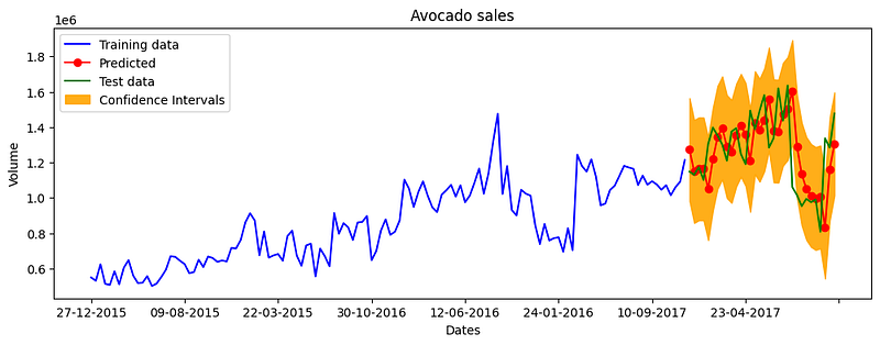
Let’s plot the outcomes and enable the model update in each iteration.

forecasts = []
confidence_intervals = []

for add_obs in test:
    fc, conf = one_period_forecast()
    forecasts.append(fc)
    confidence_intervals.append(conf)
    # Updates the existing model
    model.update(add_obs)

# Plot the results
plot_it()

# Calculate MAPE
print(f"MAPE: {mean_absolute_percentage_error(test, forecasts)}")

The plot is as below. The MAPE is 0.11918293096560012 or 11.9%. It seems not a noticeable improvement over the above ARIMA model. By the principle of model parsimony, we will use the ARIMA model rather than SARIMA in our case.

Conclusions

In this post, we reviewed the classical ARIMA and SARIMA model specifications. We learned the use of the pmdarima library to search for the optimal model automatically. We learned how statsmodels generate multi-step forecasts for ARIMA. It is worth mentioning that the lagged terms in ARIMA can be considered the features in supervised learning models. In the next chapters “A Tutorial on Tree-based Time Series Forecasting” and “A Tutorial on Multi-step Time Series Forecasts,” we will re-consider the forecasting problems with a tree-based framework, which opens a door for us to a large collection of models to pursue model accuracy.

References

Box, G. E. P., Jenkins, G. M., & Reinsel, G. C. (2015). Time series analysis: Forecasting and control (5th ed.). John Wiley & Sons.
Romano, Y., Patterson, E., & Candès, E.J. (2019). Conformalized Quantile Regression. Neural Information Processing Systems.

pmdarima/examples/stock_market_example.ipynb at master · alkaline-ml/pmdarima

A statistical library designed to fill the void in Python’s time series analysis capabilities, including the equivalent…

github.com

ARIMA Model — Complete Guide to Time Series Forecasting in Python | ML+ (machinelearningplus.com)

Exploring Auto ARIMA in Python for Multiple Time Series Forecasting | by Iqbal Rahmadhan | Medium

pmdarima/pmdarima/arima/arima.py at master · alkaline-ml/pmdarima · GitHub

Forecasting in statsmodels — statsmodels 0.15.0 (+200)