A Tutorial on the Open-source Lag-Llama for Time Series Forecasting

The open-source time series foundational model Lag-Llama [1] came on the A.I. stage shortly after the open-source large language model LLaMA [2] was released in 2023. Lag-Llama and other pre-trained time series foundational models provide an important paradigm shift. They have been pre-trained with a vast amount of time series data and have stored general data patterns for time series data of different frequencies and lengths. They can recognize unseen data patterns without extensive fine-tuning. If the large time-series foundational models were fine-tuned further, they can perform comparable predictability to those non-foundational models. If you are interested in the long history of development, see the previous chapter “From RNN/LSTM to Temporal Fusion Transformers and Lag-Llama” for the evolution up to Lag-Llama.

Here are a few things to remember before you use Lag-Llama. It is designed for univariate time series and can provide probabilistic forecasts. It uses lagged covariates and calendar-features as the inputs. It is based on the decoder-only part of LLaMA. It performs zero-shot learning (ZSL) and few shot learning.

In this chapter, we will apply it to forecast the Walmart weekly store sales data. We will go over the architecture itself. We will explain the concepts of zero-shot learning. Further, we will learn the evaluation metric for probabilistic forecasts called the Continuous Ranked Probability Score (CRPS). This chapter is organized into the following sub-topics:

• Inputs — Lagged covariates and calendar features
• The architecture of Lag-Llama
• Probabilistic forecasts
• Zero-shot learning and few-shot learning
• Use Lag-Llama to forecast the Walmart weekly store sales
• Evaluation — The Continuous Ranked Probability Score (CRPS)

The Python notebook is available via this Github link for download.

Inputs — Lagged covariates and calendar features

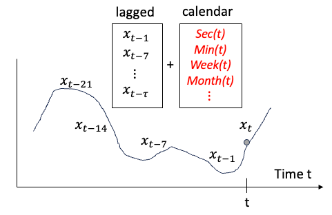
Although Large Language Models (LLMs) have their root in time series RNN/LSTM, we do not directly feed time series data to LLMs because time series data and language data are different. The time series foundational models are designed to take time series data as inputs then encode accordingly. The apparent patterns in time series data are the temporal patterns in the current and lagged values of time series. Lag-Llama uses lagged features from past values of the series to capture temporal dependencies. That’s why the model has the prefix “Lag”.

What else can we extract from time series data? We can extract date-related information such as the day of a week, the week of a month, etc. Lag-Llama adds the date-related features to the lagged covariates (t=1, 7, 14, 21, …, 𝛕) as shown in Figure (1).

Knowing the inputs, now let’s learn its architecture.

The architecture of Lag-Llama

Since Lag-Llama is based on LLaMA, and LLaMA is based on the Transformer model, it will be better to explain the evolution. LLaMA (Large Language Model Meta AI) was released by Meta AI as an open-source large language model in February 2023 (and LLaMA-2 in July 2023). LLaMA follows the Transformer architecture but replaces it with three modifications. Below I will document the prior inventions that LLaMA adopts. I will also reference those LLMs in square brackets. The three major modifications in contrast to the Transformer model are:

1. RMSNorm normalizing function [GPT3]: RMSNorm [12] was used in GPT-3 to improve the training stability. LLaMA adopts RMSNorm to normalize the input of each transformer sub-layer, instead of normalizing the output.
2. Use the SwiGLU activation function [PaLM]: Google AI presented its PaLM (Pathways Language Model) in April 2022. PaLM the SwiGLU activation function instead of the ReLU non-linearity by to improve the performance. So LLaMA adopts SwiGLU to improve performance.
3. Rotary Embeddings [GPTNeo]. The GPTNeo model is similar to GPT-2 and was released in the EleutherAI/gpt-neo Github repository. GPTNeo used the Rotary Positional Embeddings (RoPE) [11] to replace the absolute positional embeddings to achieve better performance. So LLaMA adopts RoPE.

Probabilistic forecasts

The Lag-Llama approach approximates the probabilistic forecasts by treating them as samples drawn from a Student’s t-distribution. This entails modeling three key parameters of the Student’s t-distribution: its degrees of freedom, mean, and scale. We explored the Student’s t-distribution in depth in the preceding chapter, “Monte Carlo Simulation for Time Series Probabilistic Forecasts”. Referring back to that chapter will provide a deeper understanding of the characteristics and implications of the Student’s t-distribution. Furthermore, Lag-Llama has the flexibility to incorporate other distributions besides the Student’s t-distribution.

Zero-shot learning and few-shot learning

The authors of Lag-Llama described that it has strong zero-shot performance on unseen datasets, and strong few-shot performance after they fine-tuned the model to specific data. Let’s understand what the zero-shot learning and few-shot learning are.

Zero-shot learning (ZSL) and few-shot learning (FSL) are both subfields of machine learning that focus on training models that can generalize well to new, unseen data. The key difference between the two is the number of training data, typically referred to as “shots.” ZSL assumes that the model has access to no labeled data from the target domain or task. Because the model has been trained on a large amount of labeled data, it can recognize new, unseen classes without requiring any labeled data. On the other hand, FSL assumes that the model has access to a small number of labeled data from the target domain or task.

• ZSL → No labeled data
• FSL → A small number of labeled data

Because zero-shot learning is relatively new, let’s understand it better. The basic idea behind ZSL is to learn a shared representation across multiple domains or tasks, such that the model can recognize and generalize to new classes or tasks without requiring explicit training data from those classes or tasks. This is typically achieved by using a shared embedding layer that maps input data from different domains or tasks to a common vector space, where the similarity between inputs is preserved. So let’s break down in to procedures:

1. Pre-training: The model is pre-trained on a large dataset from a related domain or task, where it learns to recognize and classify different classes or tasks.
2. Shared embedding layer: The pre-trained model is fine-tuned by adding a shared embedding layer that maps input data from different domains or tasks to a common vector space.
3. Transfer learning: The model is fine-tuned on a small number of labeled examples from the target domain or task, while freezing the shared embedding layer. This allows the model to adapt to the new domain or task while still leveraging the knowledge learned from the pre-training task.
4. Inference: Once the model is fine-tuned, it can be used to make predictions on new, unseen classes or tasks without requiring any labeled data from those classes or tasks. This is achieved by passing the input data through the shared embedding layer and then through the fine-tuned model.

Let’s delve into the data sources that Lag-Llama was trained on. Lag-Llama’s training corpus comprises 27 time series datasets spanning various domains including energy, transportation, economics, nature, air quality, and cloud operations. This diversity in the training data encompasses differences in frequencies, lengths of each series, prediction lengths, and the number of multiple series. The breadth of data sources empowers Lag-Llama with the capability of zero-shot learning.

Great. We are now ready to use Lag-Llama for our data.

Software requirement

The Lag-Llama library uses the Python gluonTS library for data formatting, forecasting, and evaluation. This is extremely convenient because we have learned the GluonTS library in the previous chapters “Amazon’s DeepAR for RNN/LSTM” and “Application: Amazon’s DeepAR for Stock Forecasts”. To save you time, I will note “same as before” in the code comments if it is the same as that in the previous chapters.

When you install gluonTS, make sure to downgrade numpy to 1.23. My platform is Google Colab.

# Same as the previous chapters"
!pip install --upgrade mxnet==1.6.0
!pip install gluonts==0.14.2
!pip uninstall numpy # Downgrade numpy to 1.23
!pip3 install mxnet-mkl==1.6.0 numpy==1.23.1

Then git clone lag-llama:

!git clone https://github.com/time-series-foundation-models/lag-llama/

And change directory to lag-llama:

cd lag-llama

You are now in “/content/lag-llama”.

You will pip install the following libraries.

# !pip install -r requirements.txt --quiet # this could take some time
# Or pip install one by one of the libraries in requirements.txt so you can observe the progress
!pip install gluonts[torch]
!pip install torch>=2.0.0
!pip install wandb
!pip install scipy
!pip install pandas==2.1.4
!pip install huggingface_hub[cli]

And download Lag_Llama from Huggingface:

!huggingface-cli download time-series-foundation-models/Lag-Llama lag-llama.ckpt --local-dir /content/lag-llama

Now we are ready to import the libraries:

from itertools import islice
from matplotlib import pyplot as plt
import matplotlib.dates as mdates
import torch
from gluonts.evaluation import make_evaluation_predictions, Evaluator
from gluonts.dataset.repository.datasets import get_dataset
from lag_llama.gluon.estimator import LagLlamaEstimator

Let’s load the Walmart data. We use the same data so we can compare the performance.

Data — The Walmart Weekly Store Sales

The historical Walmart store sales data are publicly available at Kaggle.com (https://www.kaggle.com/datasets/yasserh/walmart-dataset). This dataset has multiple weekly sales series for the stores. I have downloaded the data from Kaggle and uploaded to my google drive for Google Colab to access.

# Same as the previous chapters
%matplotlib inline
import pandas as pd
import numpy as np
from matplotlib import pyplot as plt

from google.colab import drive
drive.mount('/content/gdrive')

path = '/content/gdrive/My Drive/data/time_series'
# https://www.kaggle.com/datasets/yasserh/walmart-dataset
data = pd.read_csv(path + '/walmart2.csv') # The data have been downloaded
# convert string to datetime64
data["ds"] = pd.to_datetime(data["Date"],format='%d-%m-%Y')
#data = data.sort_values(by=['Store','ds'])
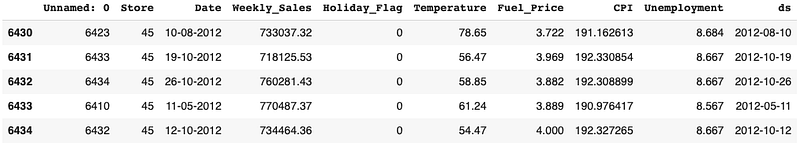
data.tail()

The dataset includes the following fields:

• Store: the unique identifier for each Walmart store
• Date: the week of sales from February 5, 2010, to November 1, 2012
• Weekly Sales: the sales amount for the specified store during the given week

Other fields include the week is a special holiday week, the temperature on the day of sale, the cost of fuel in the region where the store is located, the consumer price index, and the unemployment rate.

Let’s plot the first 5 stores.

Plot the time series

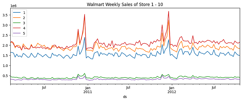
We pivot the data into the desired data shape and plot the weekly sales of the first 5 stores.

# Same as the previous chapters
# pivot the data into the correct shape
storewide = data.pivot(index='ds', columns='Store', values='Weekly_Sales')
some_stores = storewide.loc[:,1:5] # Plot only Store 1 - 5
storewide = some_stores. # Model only Store 1-10 in this demo
# plot the pivoted dataframe
some_stores.plot(figsize=(12, 4))
plt.legend(loc='upper left')
plt.title("Walmart Weekly Sales of Store 1 - 10")

You will see the co-movement among the weekly sales of the stores.

We will need to reserve some in-time data for model training and out-of-time data for model validation.

“In-time” and “out-of-time” data split

Let’s take 85% of the data as the “in-time” training data, and the rest 15% as the “out-of-time” test data.

# Same as the previous chapters
print("The time series has", storewide.shape[0], "weeks")
len_train = int(storewide.shape[0] * 0.85)
train_data = storewide[0:len_train] # 121 weeks
test_data = storewide[len_train:] # 22 weeks
[train_data.shape, test_data.shape]

The time series has 143 weeks. We take 85% as the training data and the rest as the test data. The training data have 121 weeks and the test data have 22 weeks.

Convert to GluonTS format

Any time series data should have three basic elements: the start date, the target data, and the frequency of the data. The data format of GluonTS expects these three basic elements. In the following code, we will convert our dataset to a gluonTS compatible data format. The code gets the start date by computing the minimum date, and the columns as the targets.

# Same as the previous chapters
# Prepare the data for deepAR format
from gluonts.dataset.common import ListDataset
from gluonts.dataset.field_names import FieldName

def to_deepar_format(dataframe, freq):
    start_index = dataframe.index.min()
    data = [{
                FieldName.START:  start_index,
                FieldName.TARGET:  dataframe[c].values,
            }
            for c in dataframe.columns]
    print(data[0])
    return ListDataset(data, freq=freq)
train_data_lds = to_deepar_format(train_data, 'W')
test_data_lds = to_deepar_format(test_data, 'W')

The above conversion shall work for any other time series data as well. Once it is loaded, we can start the modeling process. GluonTS requires the length of the context data for training and the length for predictions. Here we assign the length of the training data for the context and the length of the out-of-time data for prediction.

context_length = len(train_data) # 121
prediction_length = len(test_data) # 22

We are ready to use Lag-Llama for modeling.

Lag-Llama Modeling

To load and open the Lag-Llama model, we will use the following code:

ckpt = torch.load("lag-llama.ckpt", map_location=torch.device('cuda:0'))
estimator_args = ckpt["hyper_parameters"]["model_kwargs"]

Here we encounter new concepts: the .ckpt, and torch.load(). A CKPT file is a checkpoint file created by the PyTorch research framework PyTorch Lightning. The checkpoint file contains a dump of a PyTorch Lightning model. Checkpoint files contain everything needed to load the model. During model training, developers can save the current state of a model as checkpoint file, and can continue from that checkpoint to develop in the future. Another one is the PyTorch Lightning library. It is an interface for PyTorch. PyTorch is known for running deep learning experiments and later for productionizing scalable deep learning models.

We will declare the model using LagLlamaEstimator(). It requires the .ckpt file, the context and the prediction lengths, and a few other arguments as below.

estimator = LagLlamaEstimator(
    ckpt_path="lag-llama.ckpt",
    prediction_length=prediction_length,
    context_length=context_length,

    # estimator args
    input_size=estimator_args["input_size"],
    n_layer=estimator_args["n_layer"],
    n_embd_per_head=estimator_args["n_embd_per_head"],
    n_head=estimator_args["n_head"],
    scaling=estimator_args["scaling"],
    time_feat=estimator_args["time_feat"],
)

lightning_module = estimator.create_lightning_module()
transformation = estimator.create_transformation()
predictor = estimator.create_predictor(transformation, lightning_module)

With the above defined predictor(), we will use it to produce the forecasts. Remember Lag-Llama will perform Zero-shot learning (ZSL) to make predictions on the Walmart data that it may not see before.

Forecasting

We are ready to produce the forecasts.

# Same as the previous chapters
forecast_it, ts_it = make_evaluation_predictions(
    dataset=train_data_lds,
    predictor=predictor,
)

forecasts = list(forecast_it)
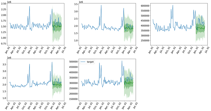
tss = list(ts_it)

Let’s visualize the predictions.

# Same as the previous chapters
plt.figure(figsize=(20, 15))
date_formater = mdates.DateFormatter('%b, %d')
plt.rcParams.update({'font.size': 15})

for idx, (forecast, ts) in islice(enumerate(zip(forecasts, tss)), 9):
    ax = plt.subplot(3, 3, idx+1)

    plt.plot(ts[-4 * dataset.metadata.prediction_length:].to_timestamp(), label="target", )
    forecast.plot( color='g')
    plt.xticks(rotation=60)
    ax.xaxis.set_major_formatter(date_formater)
    ax.set_title(forecast.item_id)

plt.gcf().tight_layout()
plt.legend()
plt.show()

Notice Lag-Llama provides the probabilistic forecasts for each time series:

Let’s see the performance.

Evaluation metrics — The continuous ranked probability score (CRPS)

In this end of this chapter, I introduce the Continuous Ranked Probability Score (CRPS). It is a popular evaluation metric when the forecasts are probabilistic forecasts rather than a point estimate. How do we evaluate the prediction performance if the predictions involve a range of probabilistic values rather than point estimates? If the outputs were point estimates, we can use mean squared error (MSE), mean absolute error (MAE), or mean absolute percentage error (MAPE). But when the outputs are probabilistic forecasts, we care about the spread of the forecasted distribution as well as the central tendency of the distribution. If the spread of the forecasted distribution is very wide such that any forecast is possible, the model cannot be considered a good model.

CRPS ranges from 0 to positive infinity. When the forecasted cumulative distribution function (CDF) perfectly matches the observed outcome, CRPS is zero. We want the CRPS to be as low as possible. The formula for the Continuous Ranked Probability Score (CRPS) is:

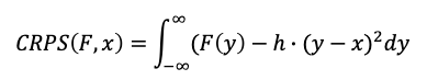
• Given a random variable x, F is the cumulative distribution function (CDF) of x, i.e,, F(y) = P(x≤y).
• h() is the Heaviside step function. It is 1.0 if x≥y, otherwise 0. It defines whether each forecasted probability exceeds the observed outcome. The Heaviside step function is simply this:

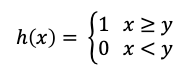
The integration in the formula means the score considers the entire range of potential outcomes and their associated probabilities.

# Same as the previous chapters
evaluator = Evaluator()
agg_metrics, ts_metrics = evaluator(iter(tss), iter(forecasts))
print("CRPS:", agg_metrics['mean_wQuantileLoss'])

The CRPS is 0.07203626685077341. It is not zero but is acceptable.

Conclusions

In this chapter we learned how to use Lag-Llama to make zero-shot predictions for our data. We learned the architecture of Lag-Llama, and the concept of zero-shot learning. Further, we will learn the evaluation metric for probabilistic forecasts called the Continuous Ranked Probability Score (CRPS).

References

• [1] Rasul, K., Ashok, A., Williams, A.R., Khorasani, A., Adamopoulos, G., Bhagwatkar, R., Bilovs, M., Ghonia, H., Hassen, N., Schneider, A., Garg, S., Drouin, A., Chapados, N., Nevmyvaka, Y., & Rish, I. (2023). Lag-Llama: Towards Foundation Models for Probabilistic Time Series Forecasting.
• [2] Touvron, H., Lavril, T., Izacard, G., Martinet, X., Lachaux, M.-A., Lacroix, T., Rozière, B., Goyal, N., Hambro, E., Azhar, F., Rodriguez, A., Joulin, A., Grave, E. & Lample, G. (2023). LLaMA: Open and Efficient Foundation Language Models (cite arxiv:2302.13971)