From RNN/LSTM to Temporal Fusion Transformers and Lag-Llama

In the previous chapter “The Progression of Time Series Modeling Techniques,” we have surveyed the connections of simple moving average, seasonal-trend decomposition, ARIMA, Kalman filter, state space model, and then RNN/LSTM/GRU. In this chapter, we will continue to learn from RNN/LSTM to Temporal Fusion Transformers and Lag-Llama. Many of today’s large language models have their roots in time series RNN/LSTM, and the Transformer framework of the paper “Attention is all you need” [2]. There are several milestones from RNN/LSTM to Transformer, including sequence-to-sequence modeling, the attention mechanism, and the self-attention mechanism (notice the self-attention and attention are different). While each of these mentioned algorithms deserves a whole chapter, this chapter aims at the landscaping view for the connection from one innovation to another. By navigating the evolution from one to another, we will have a fresh look to the innovations and be inspired for further work.

Further, since the large language models (LLMs) have their roots in the time series RNN/LSTM models, why do we need to develop time-series suitable large models? Why can’t we just use LLMs for time series modeling, or at least as effective as the time-series large models? In this chapter we will explain that. We will cover:

• From RNN/LSTM to sequence-to-sequence (Seq2Seq) learning
• The attention mechanism
• The self-attention mechanism
• The Transformer model
• Why language Transformer models may not be effective for time series
• From Transformer to Temporal Fusion Transformer
• Why are we interested in foundational models for time series?
• Lag-Llama — an open-source time series foundational model

From RNN/LSTM to Sequence-to-sequence (Seq2Seq) models

I bought my first voice translation device in the 2000s. The quality of translation was merely acceptable, but it helped me travel to Korea and Paris. If its translation quality can be better, it will benefit people around the world who speak different languages to communicate easily. In the past 20 years, many researchers have engaged to solve such a worldwide application. The early algorithms Statistical Machine Translation (SMT) and Hidden Markov Models (HMMs) used hand-crafted features such as n-grams, syntax-based features, and alignment features to translate text from one language to another. These traditional algorithms require hand-crafted features and are often brittle and difficult to train. Another challenge in language translation is varying lengths between the source sentence and the target sentence. Let’s see the following English sentence and its translation in French and Italian:

• English (15 words): “After finishing work, I often make a detour to the chocolate shop for some treats.”
• French (16 words): “Après avoir fini le travail, je fais souvent un détour par la chocolaterie pour quelques friandises.”
• Italian (18 words): “Dopo aver finito il lavoro, spesso faccio un giro di sosta al negozio di cioccolato per qualche dolcetto.”

The varying lengths tell us that language translation needs semantic comprehension rather than mechanical word-for-word translation.

The translation solution got a big leap when Ilya Sutskever, Oriol Vinyals, and Quoc V. Le published their paper “Sequence to Sequence Learning with Neural Networks” in 2014 [1]. Their neural-network framework provides the general flexibility and does not require hand-crafted, stylized features. Most of all, Seq2Seq can solve the varying-length problem effectively. Seq2Seq consists of an encoder network that encodes the input sequence into the “context vector”, and a decoder network to generates the output sequence from this vector. This strategy nicely de-couples the input sequence and the target sequence. See Figure (1).

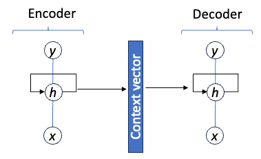
Figure (2) unrolls the encoder RNN and the decoder RNN. The context vector captures the semantic meaning of the input sequence. You can think of Seq2Seq model as a way to comprehend the information in order to translate into another language.

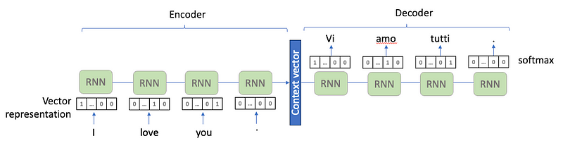
RNN/LSTM is a time series modeling tool, and now is leveraged to be a language modeling tool. There is a fundamental difference between language data and time series. Language data are words and punctuations, and time series data are just numbers. Language data have to be coded into numerical vector representation to feed into a neural network algorithm. The outputs also need to be decoded to become words. The paper [1] used 160,000 of frequently-used words for the input data. The word “I” becomes a 160,000-length vector in which the element position of “I” is 1.0 otherwise 0.0. Likewise, the word “love” is another 160,000-length vector where the element position “love” is 1.0 otherwise 0.0. You can find detail explanations for the text representation in “The Handbook of NLP with Gensim” by Kuo (2023) [3].

What do the RNN blocks do in Figure (2)? They calculate the weighted average of the previous hidden state ht-1 and their new input xt, plus a bias. The weights and biases can be considered the treasure of the model. The weights and biases of the RNN blocks are all the same regardless different input vector representations “I”, “love”, and “you”. The above RNN framework has one hidden state connecting all RNN blocks. For a long sentence, it suffers the well-known vanishing gradient problem. The vanishing gradient problem is solved by Long Short-Term Memory. Without iterating the content here, you can reference the previous chapter “The Progression of Time Series Modeling Techniques” that explains the vanishing gradient problem and how LSTM creates two hidden paths, one for the long-term memory and the other one for the short-term memory, to solve the problem. Figure (3) replaces the RNN blocks with the LSTM blocks.

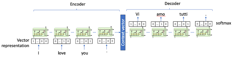
Now let’s focus on the weights and biases. The fact that they are all the same, regardless the position of a word, appears too restrictive. For example, “love” and “.” having the same weights and biases seem not natural and too restrictive. Any spoken language is magical and can have a lot of implicit connotations. By using just a set of LSTMs to encode sentences can lose a lot of information.

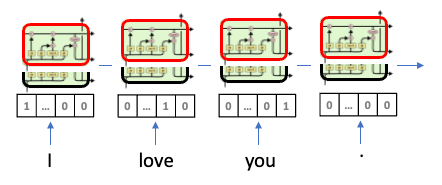
To capture more variations in the inputs, researchers add a second set of LSTMs like the black LSTMs and the red LSTMs in Figure (3). All the black LSTMs have the same weights and biases, and all the red LSTMs have the same the weights and biases and are different from those of the black LSTMs. The two sets of LSTMs thus have two sets of short-term memories and two sets of long-term memories to capture the variations in the input vectors. If needed, more layers of LSTMs can be added. Remember this concept is later borrowed in the Transformer model called the “Multi-head”.

Let’s talking about the context vector and the decoder in Figure (2). The context vector provides the initial values for the decoder. The decoder consists of LSTM blocks. All the LSTMs in the decoder have the same weights and biases but are different from those LSTMs in the encoder. Each LSTM will pass a vector to be decoded through the softmax function to be a word or a punctuation. If the sentence is shorter than the fixed length, an [EOS] (end of sentence) symbol is filled in. Thus, Seq2Seq can deal with the varying lengths in the source and target sentences.

Knowing the innovation in Seq2Seq, let’s learn its second feature — the attention mechanism.

The attention mechanism

When we listen to a sentence, we unknowingly have paid attentions to important keywords. When we hear “after finishing work, I often make a detour to the chocolate shop for some treats,” we pick up the keywords “after work” and “chocolate shop”. This special attention is the attention mechanism that focus on some parts of the input sentence. Seq2Seq works in the same way. It pays more attention to those words to render them into the target language.

A major drawback in the “one-pipeline” architecture in Figure (3) is that the encoder needs to represent the entire input sentence in the single hidden state vector ht. This can cause information loss because all information need to be compressed into the hidden state ht. Further, the decoder needs to decipher the information from the single vector only. One of the seminal papers that introduced attention mechanisms in the context of Seq2Seq models is “Neural Machine Translation by Jointly Learning to Align and Translate” by Dzmitry Bahdanau, Kyunghyun Cho, and Yoshua Bengio in 2015 [4]. They designed an attention mechanism to allow the decoder to focus on relevant parts of the input sequence at each decoding step. This work laid the foundation for many subsequent developments in sequence-to-sequence modeling with attention mechanisms.

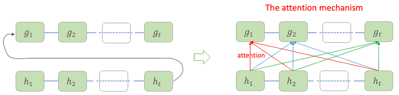
Figure (4) shows the one-pipeline architecture in the left is replaced by the attention mechanism in the right. At each time step during decoding, the decoder generates a hidden state (gt) based on the previous hidden state and the previously generated token. Then the attention mechanism computes attention weights for each position in the input sequence. These weights indicate the relevance or importance of each input token to the current decoding step. Using the attention weights, a context vector is calculated as a weighted sum of the encoder states. This context vector is then combined with the current decoder state to generate the output token for the current time step.

Let’s summarize the key points. Encoding is like a person reading or in-taking information. Decoding is like this person speaking up using his/her own words. When we speak with words, we may pay more attention to some key words we have read and depict accordingly. The attention mechanism lets the model to assign different weights to some parts of the input sequence when producing an output sequence.

A special type of attention mechanism, called self-attention, is proven to be more effective. Let’s see what it is.

From attention to self-attention

Self-attention, also known as intra-attention, is a specific type of attention mechanism. The term “self” in self-attention emphasizes that the attention mechanism operates internally within the same sentence rather than attending to external sentences. This mechanism has proven to be highly effective in various natural language processing tasks. This was proposed in the seminal paper “Attention is All You Need” (2017) [2].

Figure (5) shows a self-attention example by a popular app bertviz. In the sentence “The rabbit quickly hopped, the turtle slowly crawled,” the word “rabbit” is more related to “hopped”, and the word “turtle” is related to “crawled”. The thickness of the lines between words indicate the strength of the relationships. When the word “rabbit” appears, there is a higher chance to predict “hopped”, likewise “turtle” to predict “crawled”.

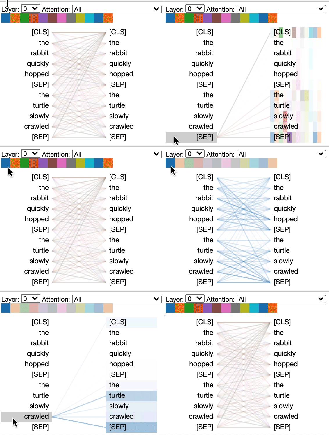
To compute self-attention, the input embeddings are transformed into three kinds of vectors: query vectors, key vectors, and value vectors. These transformations are typically linear projections, learned parameters of the model. For each token in the same sentence, an attention score is computed by taking the dot product between its query vector and the key vectors of all tokens in the sentence.

The Transformer Model

The Transformer model has revolutionized natural language processing tasks due to its attention mechanism-based architecture. Figure (6) shows the Transformer architecture:

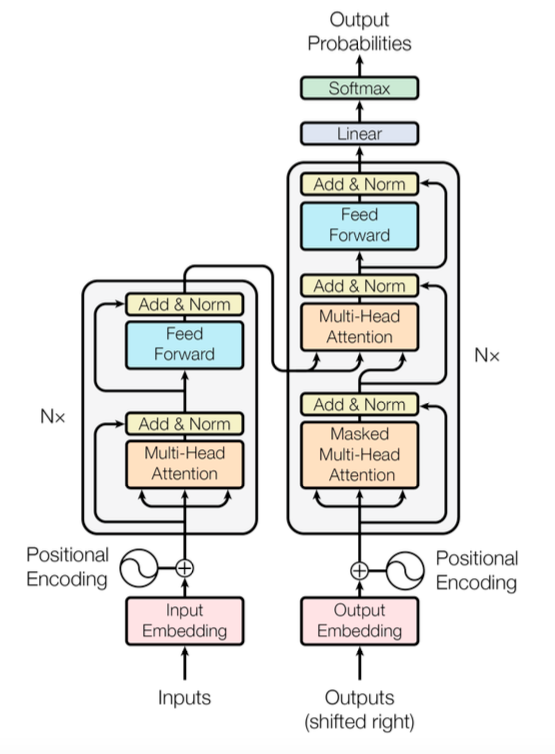
1. Input Embeddings: The input to the Transformer model consists of tokenized input sequences. Each token is initially represented as a fixed-dimensional vector like explained in Figure (2).
2. Positional Encodings: Suppose you have a sentence like “I love ice cream”. In a transformer model, we don’t want it to just understand “I”, “love”, and “ice cream” as individual words. We also want it to understand that “I” comes first, then “love”, and then “ice cream”. When you read a sentence, you naturally understand the meaning based not only on the words themselves but also on their order in the sentence. Similarly, in a transformer model, we need a way to tell the model about the position of each word or token in a sequence. The positional encodings are like little tags attached to each word or token in the sequence, telling the model about its position in the sequence. So, the transformer can use both the words themselves and these positional tags to understand the input better.
3. Multi-Head Self-Attention Mechanism: we already learned the “self-attention” in the previous section, which means paying attention to some parts within the same sentence. But what is “multi-head”? In Figure (3) we already have this idea. Here, similarly, instead of computing attention only once, the model can computes attention multiple times in parallel, each with its own set of learned linear projections. These parallel computations are referred to as “attention heads.”
4. Fully Connected Feed-Forward Network: This is a standard neural network. The term “fully connected” indicates that every neuron in a layer is connected to every neuron in the subsequent layer. The term “feed-forward” refers to the flow of data through the network without any feedback loops.

The decoder stack, in the right hand side of Figure (6), is similar to the encoder stack but contains an additional self-attention layer that attends to the encoder’s output. This enables the decoder to focus on relevant parts of the input sequence while generating the output sequence. The final layer is a softmax function to generate the output probability distribution over the target vocabulary.

Other than the above, the model is trained using standard backpropagation and stochastic gradient descent (SGD) optimization with the Adam optimizer. During training, both the encoder and decoder are trained jointly to minimize the cross-entropy loss between the predicted and target sequences.

Why language transformer models may not be effective for time series

Several reasons explain why language transformer models may not effective for time series data. The first reason is that time series often exhibit complex temporal patterns and dependencies that span across multiple time steps. Without significant modifications, transformer models may not capture the temporal patterns effectively.

The second reason is the calendar-related patterns in time series data. The calendar-related patterns may not be explicitly captured by standard Transformer architectures.

The length of the inputs is the third reason. Transformers typically apply fillers to standardize sequences to fixed lengths. Time series data, on the other hand, can have variable lengths depending on the length of the time series. Adapting the Transformer architecture to handle varying length inputs requires additional modifications or techniques. The fourth reason is the need for prediction uncertainty in time series. language models typically do not have it.

With the above reasons, researchers have been exploring adaptations and extensions to the transformer models to make them more effective for time series modeling. A significant milestone model is the Temporal Fusion Transformer (TFT).

From Transformer to Temporal Fusion Transformer (TFT)

Time series data and language data are different. A direct application of the Transformer model for time series data will not be effective without signification modifications. In 2020, Bryan Lim, Sercan O ̈. Arık, Nicolas Loeff, and Tomas Pfister proposed a seminal paper “Temporal Fusion Transformers for Interpretable Multi-horizon Time Series Forecasting” for multi-series and multi-period time series modeling [5].

Let’s start with how to get features for multiple time series data. Time series data possess temporal patterns between current and lagged values. Time series data also have calendar-related information. The calendar features such as the day of a week or the week of a month, are deterministic even in the future. So TFT creates four broad types of features. Let me explain the four feature groups with the Walmart store sales data in the previous chapter “Amazon’s DeepAR for RNN/LSTM”:

• (Feature group 1) Past covariates of a store: The past sales yt-1, yt-2, …, of a store i. This is time-varying known only up to time t.
• (Feature group 2) Other data that influence the store sales: Such as weather or the consumer index. This is time-varying only known up to time t.
• (Feature group 3) Calendar features such as the day in a week, the week in a month, or holidays.
• (Feature group 4) Time-invariant features such as store ID or regions that are not related with time.

TFT leverages self-attention mechanisms to capture complex temporal dependencies within the data. To capture the temporal nature of time series data, the authors introduce temporal encoding techniques. These techniques allow the model to incorporate time-related information into the input sequence, enabling better capture of temporal patterns and trends. Knowing the autoregressive patterns in time series, TFT utilizes an autoregressive mechanism for generating multi-horizon forecasts.

In addition to the Transformer architecture, several contributions made TFT an appealing choice. One of the key contributions of TFT is its emphasis on interpretability. The authors introduce attention mechanisms that highlight the importance of different input features and temporal components, making the forecasts more interpretable and transparent to users. TFT provides estimates of uncertainty along with the forecasts, which is crucial for decision-making under uncertainty. By quantifying the uncertainty associated with each prediction, the model can provide more reliable forecasts and guide risk management strategies. TFT is capable of producing multi-horizon forecasts, predicting future values at multiple time steps ahead. Finally, TFT designed to handle time series data with missing or sparse observations effectively. It can learn from incomplete data and make forecasts even when some observations are missing, which is common in real-world time series datasets.

We do not plan to go deep for TFT In this overview chapter. We will learn more detail about the TFT architecture and its visualization in the next chapters.

Why are we interested in foundational models for time series?

Large foundational models are trained on massive amount of data for general uses. They can be fine-tuned for specific tasks. In language models, you may have heard of GPT-2 (2019), GPT-3 (2020), chatGPT (2022), GPT-4 (2023), T-5 (2019), Flan-T5 (2022), BERT (2018), RoBERTa (2019), DeBERTa (2019), DistilBERT (2020), and MPT-7B-StoryWriter-65k+. These models have learned the nuances of language effectively, including grammar, semantics, and context. In the post “The data that those large language models were built on” [6], I detailed the data sources such as books and articles, and internet posts to train those models.

Why are we interested in large foundational models for time series? Here let me offer several good motivations. A pre-trained time series foundational model is already trained on a diverse amount of time series data in finance, healthcare, or astronomical science to recognize general patterns. They are able to recognize the patterns in unseen time series without extensive fine-tuning. Their flexibility allows them to handle data types of different industries, sampling frequencies, and forecasting horizons. Foundational models in time series can reduce the need for task-specific model development and speeding up deployment. Another advantage is their capability for prediction interpretability. Many large foundational models already incorporated interpretability mechanisms, allowing users to understand how the model makes predictions and forecasts.

Lag-Llama— an open-source time series foundational model

The Lag-Llama model is based on the decoder part of the LLaMA model and trained on diverse corpus of time series data. It is a general-purpose foundational model for univariate probabilistic forecasting. The reason it adds “Lag” as prefix to LLaMA is because it uses the lag terms of time series as covariates. Lag-Llama uses lagged features from past values of the series to capture temporal dependencies without assuming linearity or stationarity.

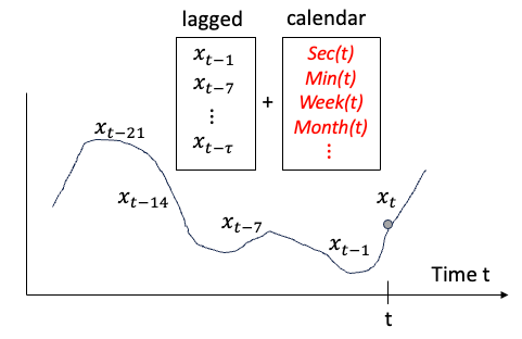
Apparently, there are differences in time series data and language data. There are temporal patterns in the current and lagged values of time series. Time series data also have calendar-related information such as the day of a week, the week of a month, etc. So Lag-Llama employs its inputs as the lagged covariates (t=1, 7, 14, 21, …, 𝛕) and the calendar-related features like shown in Figure (6). Because time series data require very different ways in encoding the inputs, it is why Lag-Llama uses the decoder part of the LLaMA model.

Lag-Llama approximates the probabilistic outputs as the results drawn from a Student’s t-distribution. So it models the three parameters of a Student’s t-distribution, namely its degrees of freedom, mean, and scale. We have studied the Student’s t-distribution in the previous chapter “Monte Carlo Simulation for Time Series Probabilistic Forecasts”. You can reference it to understand the Student’s t-distribution. Other distributions can be included in Lag-Llama as well.

Since Lag-Llama is based on LLaMA, and LLaMA is based on the Transformer model, it will be better to explain the evolution. LLaMA (Large Language Model Meta AI) was released by Meta AI as an open-source large language model in February 2023 (and LLaMA-2 in July 2023). LLaMA follows the Transformer architecture but replaces it with three modifications. Below I will document the prior inventions that LLaMA adopts. I will also reference those LLMs in square brackets. The three major modifications in contrast to the Transformer model are:

1. RMSNorm normalizing function [GPT3]: RMSNorm [12] was used in GPT-3 to improve the training stability. LLaMA adopts RMSNorm to normalize the input of each transformer sub-layer, instead of normalizing the output.
2. Use the SwiGLU activation function [PaLM]: Google AI presented its PaLM (Pathways Language Model) in April 2022. PaLM the SwiGLU activation function instead of the ReLU non-linearity by to improve the performance. So LLaMA adopts SwiGLU to improve performance.
3. Rotary Embeddings [GPTNeo]. The GPTNeo model is similar to GPT-2 and was released in the EleutherAI/gpt-neo Github repository. GPTNeo used the Rotary Positional Embeddings (RoPE) [11] to replace the absolute positional embeddings to achieve better performance. So LLaMA adopts RoPE.

Let’s understand the data sources that it was trained on. Lag-Llama uses a corpus of 27 time series datasets from domains such as energy, transportation, economics, nature, air quality and cloud operations. The variety in the training data such as frequencies, lengths of each series, prediction lengths, number of multiple series. The diverse data sources enable Lag-Llama to model new time series that it hasn’t been explicitly trained on. This is called the Zero-shot learning. The zero-shot learning is a new learning approach that a model is trained to recognize classes it has never seen before during training.

Conclusions

In this chapter, we went through the evolution of time series modeling techniques, tracing the path from RNN/LSTM to Temporal Fusion Transformer and Lag-Llama. We covered the sequence-to-sequence (Seq2Seq) model, the attention mechanism, the self-attention mechanism, and the Transformer model. We explained why language Transformer models may not be effective for time series. Then we introduced Temporal Fusion Transformer (TFT) that incorporates temporal encoding techniques and emphasizes interpretability and uncertainty estimation. Finally, we learned Lag-Llama, an open-source foundational model designed for univariate probabilistic time series forecasting.

In the next few chapters, we will learn Temporal Fusion Transformer including how it visualizes time series models for interpretability. We will also build time series models with Lag-Llama.

References

• [1] Sutskever, I., Vinyals, O. & Le, Q. V. (2014). Sequence to sequence learning with neural networks. Advances in neural information processing systems (p./pp. 3104–3112)
• [2] Vaswani, A., Shazeer, N., Parmar, N., Uszkoreit, J., Jones, L., Gomez, A. N., Kaiser, Ł. & Polosukhin, I. (2017). Attention is all you need. Advances in Neural Information Processing Systems (p./pp. 5998–6008).
• [3] Kuo, C. (2023). The Handbook of NLP with Gensim: Leverage topic modeling to uncover hidden patterns, themes, and valuable insights within textual data. Packt Publishing. ISBN-13: 978–1803244945
• [4] Bahdanau, D., Cho, K., & Bengio, Y. (2014). Neural Machine Translation by Jointly Learning to Align and Translate. CoRR, abs/1409.0473.
• [5] Lim, Bryan & Arık, Sercan Ö. & Loeff, Nicolas & Pfister, Tomas, 2021. “Temporal Fusion Transformers for interpretable multi-horizon time series forecasting,” International Journal of Forecasting, Elsevier, vol. 37(4), pages 1748–1764.
• [6] Kuo, C., (2023). The data that those large language models were built on. Medium.com
• [7] Rasul, K., Ashok, A., Williams, A.R., Khorasani, A., Adamopoulos, G., Bhagwatkar, R., Bilovs, M., Ghonia, H., Hassen, N., Schneider, A., Garg, S., Drouin, A., Chapados, N., Nevmyvaka, Y., & Rish, I. (2023). Lag-Llama: Towards Foundation Models for Probabilistic Time Series Forecasting.
• [8] Touvron, H., Lavril, T., Izacard, G., Martinet, X., Lachaux, M.-A., Lacroix, T., Rozière, B., Goyal, N., Hambro, E., Azhar, F., Rodriguez, A., Joulin, A., Grave, E. & Lample, G. (2023). LLaMA: Open and Efficient Foundation Language Models (cite arxiv:2302.13971)
• [9] Chowdhery, A., Narang, S., Devlin, J., Bosma, M., Mishra, G., Roberts, A., Barham, P., Chung, H.W., Sutton, C., Gehrmann, S., Schuh, P., Shi, K., Tsvyashchenko, S., Maynez, J., Rao, A., Barnes, P., Tay, Y., Shazeer, N.M., Prabhakaran, V., Reif, E., Du, N., Hutchinson, B.C., Pope, R., Bradbury, J., Austin, J., Isard, M., Gur-Ari, G., Yin, P., Duke, T., Levskaya, A., Ghemawat, S., Dev, S., Michalewski, H., García, X., Misra, V., Robinson, K., Fedus, L., Zhou, D., Ippolito, D., Luan, D., Lim, H., Zoph, B., Spiridonov, A., Sepassi, R., Dohan, D., Agrawal, S., Omernick, M., Dai, A.M., Pillai, T.S., Pellat, M., Lewkowycz, A., Moreira, E., Child, R., Polozov, O., Lee, K., Zhou, Z., Wang, X., Saeta, B., Díaz, M., Firat, O., Catasta, M., Wei, J., Meier-Hellstern, K.S., Eck, D., Dean, J., Petrov, S., & Fiedel, N. (2022). PaLM: Scaling Language Modeling with Pathways. J. Mach. Learn. Res., 24, 240:1–240:113.
• [10] Shazeer, N.M. (2020). GLU Variants Improve Transformer. ArXiv, abs/2002.05202.
• [11] Su, J., Lu, Y., Pan, S., Wen, B., & Liu, Y. (2021). RoFormer: Enhanced Transformer with Rotary Position Embedding. ArXiv, abs/2104.09864.
• [12] Zhang, B., & Sennrich, R. (2019). Root Mean Square Layer Normalization. ArXiv, abs/1910.07467.