
Amazon’s DeepAR for RNN/LSTM

New real-world use cases bring forth new technical innovations. Let’s consider two use cases. An electricity company needs to forecast the energy consumptions of each of the thousands or millions of households in a geographical area. The predictions can enable the electricity company to plan and allocate resources at household level. The electricity company also needs the prediction uncertainty so the company can plan with more certainty. The second use case happens in e-commerce businesses (like Amazon.com). They need to forecast the inventories of individual products for planning. They needs to know the prediction uncertainty. They even need the forecasts for new products that have no historical data.
These use cases demand new modeling techniques that can forecast multiple periods but not just one period. The new techniques should forecast multiple related time series all together. The new techniques should provide the prediction range but not just one predicted value. In short, the new techniques should provide multi-step forecasts, multi-series forecasts, and forecasts with uncertainty.
We have learned RNN/LSTM in the previous chapter “The History of Time Series Modeling Techniques”. In this chapter we will introduce the DeepAR framework. The DeepAR framework is an autoregressive recurrent networks (RNNs) proposed by Salinas et. al. (2020) [2]. The DeepAR framework meets the need for multi-step-ahead forecasts because of its deep learning framework. It also meets the need for multi-series forecasting, again, because of its deep learning framework. DeepAR provides the capacity to forecast uncertainty. In the above electricity consumption and e-commerce product examples, the vast amount of time series data can increase the prediction accuracy without overfitting. Also, the co-forecasting technique even can produce the predictions for new products when past data are not available. The DeepAR model is engineered in the GluonTS library, a popular library open-sourced by the team at Amazon [1]. These appealing features invite us to learn and adopt gluonTS to more use cases.
In this chapter, we will learn the following topics:
- From a local model to a global model
- DeepAR estimates the probability distribution
- Understanding the engineering of GluonTS
- Data Preparation in GluonTS
- Modeling in GluonTS
- Forecasting in GluonTS
After reading this chapter, you will be able to build models for multi-period forecasts, multi-series forecasts, and prediction uncertainty. The Python Notebook is available here for you to download. So let’s start with DeepAR.
From a local model to a global model
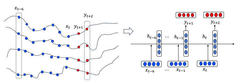
If a model deals with a single time series, it is called a local model. If a model is developed on multiple time series and the parameters are shared by all the time series, the model is called a global model. A node in the deep learning model is a data point of a time series, the model deals with an univariate time series. And if the node is extended to be a vector, the model is dealing with multiple time series. So such extension from local to global is straightforward in a neural network framework. The following diagram shows the idea. Assume there are four time series. The values of the four time series at time t form a vector of four elements. The right hand side of the diagram is the RNN in vector form. The global model applies the same parameters for the four time series.
DeepAR estimates the probability distribution
Rather than predicting a single point, DeepAR assumes a prediction comes from a distribution. It estimates the parameters of a distribution such as the mean and the standard deviation of a Gaussian distribution. This allows DeepAR to produce the prediction uncertainty, which consists of the forecasts from a range of possible values. The generation of possible values from a given distribution is actually the classical Monte Carlo simulation. I include a short description and code for the Monte Carlo simulation if you can use some help.
Let’s see how DeepAR assumes the observed values coming from a distribution. Assume the distribution is a Gaussian distribution with mean µ and standard deviation 𝜎. DeepAR can derive the likelihood function p(z|µ,𝜎) as Equation (1):

Where the mean and standard deviation of the Gaussian distribution are functions of the hidden parameter hi,t:
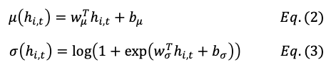
The weight parameters 𝑤 in Eq. (2) and (3) respectively are to be estimated, and b_u and b_𝜎 are random noises.
Understanding the engineering of GluonTS
Since 2020, the Gluon Time Series Toolkit (GluonTS) has been used for complex deep-learning-based time series modeling tasks [1]. GluonTS has streamlined the data preparatory steps that often involve not trivial data wrangling job. GluonTS provides the tools for quick model development, efficient experimentation and evaluation. It helps us to deliver reproducible results after the proof-pf-concept models. In addition to its neural network frameworks, it includes classical models, such as ARIMA and ETS.
It will be helpful to mention the engineering design of this library. The core design principles of GluonTS are: modularity, scalability, and reproducibility. Firstly, modularity is ingrained within the codebase. GluonTS splits down the system into small, discrete components with clearly defined interfaces. This architecture empowers data scientists to construct models with flexibility and ease. Secondly, scalability is another key feature. GluonTS can handles datasets of varying sizes without straining system resources. This is achieved through the adept use of Python iterators, facilitating data streaming within our processing APIs. As a result, there’s no need to load entire datasets into memory, ensuring efficient utilization of computational resources. Lastly, reproducibility is important to the scientific process. With GluonTS, all experiment details are logged, including parameter values and configurations. This means that an experiment can be recreated for verification and refinement.
Great. Having learned GluonTS, let’s start to do modeling. We will talk about software first.
Software requirement
When you install gluonts, make sure to downgrade numpy to 1.23.
# Installation of gluonTS
!pip install --upgrade mxnet==1.6.0
!pip install gluonts==0.14.2
!pip uninstall numpy # Downgrade numpy to 1.23
!pip3 install numpy==1.23.1
For interested readers, you can take a look of the autogluon library (https://auto.gluon.ai) is an AutoML aims at all Text, Image, and Tabular Data. It includes the gluonts functions. Autogluon is not needed in this chapter.
Next, let’s load the data.
Store sales data
We will use the historical Walmart store weekly sales data publicly available at Kaggle.com (https://www.kaggle.com/datasets/yasserh/walmart-dataset). We choose this dataset because it has the time series for multiple stores, which enable us to demonstrate the power of gluonTS. I have downloaded the data from Kaggle and uploaded to my google drive for Google Colab to access.
%matplotlib inline
import pandas as pd
import numpy as np
from matplotlib import pyplot as plt

from google.colab import drive
drive.mount('/content/gdrive')

path = '/content/gdrive/My Drive/data/time_series'
# source: https://www.kaggle.com/datasets/yasserh/walmart-dataset
data = pd.read_csv(path + '/walmart.csv')
# convert string to datetime64
data["ds"] = pd.to_datetime(data["Date"])
data = data.sort_values(by=['Store','ds'])
data.tail()
The dataset includes the following fields:
- Store: the unique identifier for each Walmart store
- Date: the week of sales from February 5, 2010, to November 1, 2012
- Weekly Sales: the sales amount for the specified store during the given week
Other fields include the week is a special holiday week, the temperature on the day of sale, the cost of fuel in the region where the store is located, the consumer price index, and the unemployment rate.
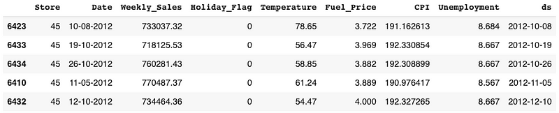
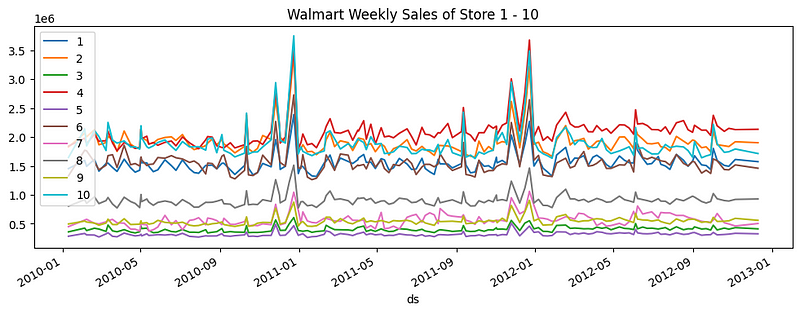
We will just use the date and weekly sales in this chapter. Let’s pivot the data into the desired data shape and plot the weekly sales of the first 10 stores.
# pivot the data into the correct shape
storewide = data.pivot(index='ds', columns='Store', values='Weekly_Sales')
some_stores = storewide.loc[:,1:10] # Plot only Store 1 - 10
# plot the pivoted dataframe
some_stores.plot(figsize=(12, 4))
plt.legend(loc='upper left')
plt.title("Walmart Weekly Sales of Store 1 - 10")
You will see the co-movement among the weekly sales of the stores.
We will take 85% of the data as the “in-time” training data, and the rest 15% as the “out-of-time” test data.
print("The time series has", storewide.shape[0], "weeks")

len_train = int(storewide.shape[0] * 0.85)
train_data = storewide[0:len_train]
test_data = storewide[len_train:]
[train_data.shape, test_data.shape]
The data has 45 columns for 45 stores. There are 121 weeks in the training data and 22 weeks in the test data. Let’s learn the data preparation class in GluonTS.
Data Preparation in GluonTS
Any time series data should have three basic elements: the start date, the target data, and the frequency of the data. The data format of GluonTS expects these three basic elements. In the following code, we will convert our dataset to a gluonTS compatible data format. The code gets the start date by computing the minimum date, and the columns as the targets.
# Prepare the data
from gluonts.dataset.common import ListDataset
from gluonts.dataset.field_names import FieldName

def to_deepar_format(dataframe, freq):
    start_index = dataframe.index.min()
    data = [{
                FieldName.START:  start_index,
                FieldName.TARGET:  dataframe[c].values,
            }
            for c in dataframe.columns]
    print(data[0])
    return ListDataset(data, freq=freq)

train_data_lds = to_deepar_format(train_data, 'W')
test_data_lds = to_deepar_format(test_data, 'W')
The above conversion shall work for any other time series data as well. Once it is loaded, we can start the modeling process.
Modeling with GluonTS
The modeling code has quite succinct lines. The code below uses the DeepAREstimator() function and I will explain accordingly.
# api: https://ts.gluon.ai/stable/api/gluonts/gluonts.mx.model.deepar.html
# paper: Salinas, David, Valentin Flunkert, and Jan Gasthaus. “DeepAR: Probabilistic forecasting with autoregressive recurrent networks.” arXiv preprint arXiv:1704.04110 (2017).

from gluonts.mx.model.deepar import DeepAREstimator
from gluonts.mx.trainer import Trainer

prediction_length = 11
context_length = 11
num_cells = 32
num_layers = 2
epochs= 5
freq="W" # Our data is weekly

estimator =   DeepAREstimator(freq=freq,
                                context_length=context_length,
                                prediction_length=prediction_length,
                                num_layers=num_layers,
                                num_cells=num_cells,
                                trainer=Trainer(epochs=epochs))
predictor = estimator.train(train_data_lds)
Let’s review the key hyper-parameters.
- freq — The frequency of the data to train on and predict. For example, our data is “W” for weekly.
- prediction_length — This is the length of the prediction horizon.
- context_length — This is the number of steps to unroll the RNN for before computing predictions. Typically it is set the same as the above prediction length. So the default is context_length = prediction_length.
- num_layers — This is the number of RNN layers. The default is 2.
- Epoch — An epoch is the entire passing of training data through the algorithm.
One implicit dependency of GluonTS is PyTorch. PyTorch is a great open-source product for neural network frameworks. The DeepAREstimator function lets you provide the hyper-parameters to the Trainer() function in PyTorch. That’s what the trainer=Trainer(epochs=epochs) is about. Further, because this is a neural network model, you have the control of the neural network hyper-parameters. I just list a few of them below.
- hidden_size — This is the number of RNN cells for each layer. The default is 40.
- lr — This is the learning rate. The default is
1e-3. - weight_decay — This is the weight decay regularization parameter. The default is
1e-8. - dropout_rate — This is the dropout regularization parameter. The default is 0.1.
Once the modeling task completes, let’s make the forecasts.
Forecasting in GluonTS
When we validate a time series model, we make the forecasts in the out-of-time or test window and use the test data to validate the forecasting performance. This standard procedure is nicely programmed in the function make_evaluation_prediction. It predict the last window of the test data and evaluate the model performance accordingly. Specifically, it does the following steps:
- It removes the final window of length
prediction_lengthof the test data. - Then it uses the remaining test data to make predictions.
- Then it compares the predictions to the actual values in the final window of length.
In our case, we want 11 weeks as the prediction length.
from gluonts.evaluation.backtest import make_evaluation_predictions
forecast_it, ts_it = make_evaluation_predictions(
    dataset=test_data_lds,
    predictor=predictor,
)
tss = list(ts_it)
forecasts = list(forecast_it)
A great feature of gluonTS is its capacity to provide probabilistic forecasts. Let’s understand how it works.
Probabilistic forecasts
In GluonTS, probabilistic forecasts are provided through probability distributions. These distributions represent the uncertainty associated with future predictions, allowing users to quantify the range of possible outcomes. GluonTS performs the Monte Carlo simulation as explained in the previous DeepAR section. The common distribution is the Gaussian Distribution. It is characterized by two parameters: the mean (μ) and the standard deviation (σ), which determine the central tendency and spread of the distribution, respectively. GluonTS predicts the mean and standard deviation of the Gaussian distribution. The predicted mean represents the point forecast, while the standard deviation represents the uncertainty around the prediction. Several other types of probability distributions used by gluonTS are Student’s t-Distribution, Negative Binomial Distribution, and Gamma Distribution.
Let’s visualize the predictions.
Graphic outcomes
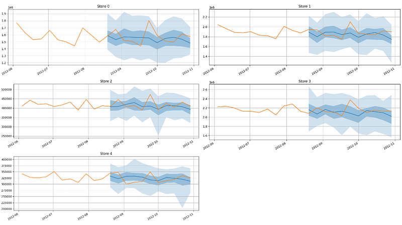
While the multiple time series were modeled and forecasted together, we can plot each individual time series. I will just plot the time series of the first 5 stores:
for k in range(5): #len(forecasts)):
  fig, ax1 = plt.subplots(1, 1, figsize=(12, 4))
  forecasts[k].plot(ax = ax1)
  tss[k].plot(ax = ax1)
  ax1.get_legend().remove()
  plt.grid(which="both")
  plt.title("Store " + str(k) )
  plt.show()
The dark blue shaded area is the 50% confidence intervals, and the light blue area is the 95%.
Now let’s inspect the evaluation metrics.
Evaluation metrics
The evaluation function produces the standard evaluation metrics. We are familiar with the evaluation metrics including MAPE, MSE for an univariate time series. The evaluation metrics for multiple time series are just the average performances of multiple time series.
from gluonts.evaluation import Evaluator

evaluator = Evaluator()
agg_metrics, item_metrics = evaluator(iter(tss), iter(forecasts), num_series=len(test_data_lds))

import json
print(json.dumps(agg_metrics, indent=4))- “MSE”: 8200494702.157576,
- “MASE”: 1.2103036035084258,
- “MAPE”: 0.06332899879927588,
- “sMAPE”: 0.06257073337381538
Conclusions
This chapter described the demand for new modeling techniques for multi-step forecasts, multi-series forecasts, and forecasts with uncertainty. In this chapter we learned DeepAR and the gluonTS library. We highlighted the RNN/LSTM framework and its use of Monte Carlo technique for the forecasting of uncertainty. We reviewed the engineering design of GluonTS. We demonstrated the modeling and forecasting outcomes for the real-world Walmart store sales data.
In next chapter, we will perform an application to the stock predictions of a group of stocks.
Appendix: Monte Carlo Simulation
Monte Carlo (MC) simulations are named after the Monte Carlo casino in Monaco. The casino wanted to know the possible outcomes given a range of input values. Its goal is to simulate all possible paths (using random sampling) in order to find the most likely or theoretical solution. MC simulation has been applied in finance, engineering, physics extensively. In finance, MC simulation is used to model various market scenarios and assess the potential outcomes. In engineering, it is used to analyze the structural integrity of a building, or the reliability of a bridge.
Let’s describe how it works step by step:
- Step 1: an input value is randomly chosen for each task within the predetermined range of estimates.
- Step 2: an outcome is computed using this randomly selected value. Record the outcome.
The above two steps are iterated for hundreds or thousands of times. Each iteration has a distinct randomly selected values.
Because MC is used extensively in finance, I will demonstrate how it is used to simulate stock prices. Here we load Apple’s daily stock prices from 2020 to 2024.
import yfinance as yf
orig = yf.download(["AAPL"], start="2020-01-01", end="2024-12-31")
orig = orig[('Adj Close')]
orig.tail()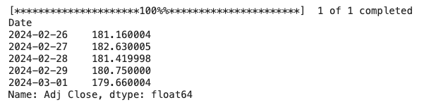
Then we calculate the simple daily returns and plot in a histogram.
import pandas as pd
import numpy as np
import matplotlib.pyplot as plt
returns = orig.pct_change()
last_price = orig[-1]
returns.hist(bins=100)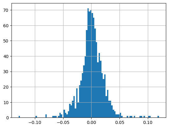
We will first calculate the historical volatility of the stock over a certain period. This is typically done by computing the standard deviation of the stock’s daily returns. We assume the future volatility will be similar to the historical volatility. The histogram looks like a normal distribution centering at 0.0. For simplicity, we assume this distribution is a standard Gaussian distribution with mean =0 and standard deviation. Below we derive the standard deviation which is also called the daily volatility. Then the daily return % for tomorrow is expected to be a random value from the Gaussian distribution:
daily_volatility = returns.std()
rtn = np.random.normal(0, daily_volatility)
The next day price is today’s price multiplying by (1+return %):

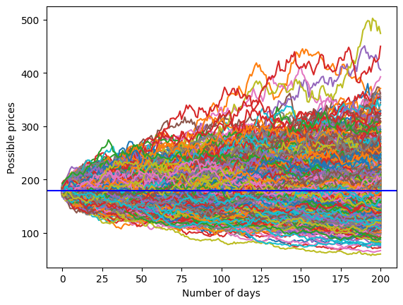
price = last_price * (1 + rtn)The above are the basic financial formula for stock prices and returns. We are going to apply the MC simulation. With tomorrow’s price, we can continue to draw randomly another return % to derive the day after tomorrow’s price. In this way we can derive a possible price path for the next, say, 200 days. But this is just a possible price path for the next 200 days. We can replicate this process 1,000 times to generate 1,000 price paths.
import warnings
warnings.simplefilter(action='ignore', category=pd.errors.PerformanceWarning)

num_simulations = 1000
num_days = 200
simulation_df = pd.DataFrame()

for x in range(num_simulations):
    count = 0

    # The first price point
    price_series = []
    rtn = np.random.normal(0, daily_volatility)
    price = last_price * (1  + rtn)
    price_series.append(price)

    # Create each price path
    for g in range(num_days):
        rtn = np.random.normal(0, daily_volatility)
        price = price_series[g] * (1  + rtn)
        price_series.append(price)

    # Save all the possible price paths
    simulation_df[x] = price_series

fig = plt.figure()
plt.plot(simulation_df)
plt.xlabel('Number of days')
plt.ylabel('Possible prices')
plt.axhline(y = last_price, color = 'b', linestyle = '-')
plt.show()
The plot looks like this. The price starts at 179.66. After 200 days, the MC simulation tells us the price can be as high as $500 or as low as $100.
And suppose we want to know the possible price range that will happen 90% of the time (between 5% and 95%), we can use quantile to get the upper and the lower bounds.
upper = simulation_df.quantile(.95, axis=1)
lower = simulation_df.quantile(.05, axis=1)
stock_range = pd.concat([upper, lower], axis=1)

fig = plt.figure()
plt.plot(stock_range)
plt.xlabel('Number of days')
plt.ylabel('Possible prices')
plt.axhline(y = last_price, color = 'b', linestyle = '-')
plt.show()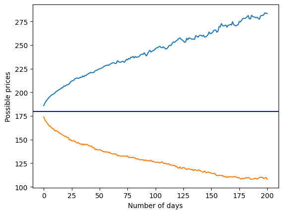
References
- [1] Alexander Alexandrov, Konstantinos Benidis, Michael Bohlke-Schneider, Valentin Flunkert, Jan Gasthaus, Tim Januschowski, Danielle C. Maddix, Syama Rangapuram, David Salinas, Jasper Schulz, Lorenzo Stella, Ali Caner Türkmen, & Yuyang Wang. (2019). GluonTS: Probabilistic Time Series Models in Python. https://www.jmlr.org/papers/volume21/19-820/19-820.pdf
- [2] David Salinas, Valentin Flunkert, Jan Gasthaus, & Tim Januschowski (2020). DeepAR: Probabilistic forecasting with autoregressive recurrent networks. International Journal of Forecasting, 36(3), 1181–1191. https://www.sciencedirect.com/science/article/pii/S0169207019301888


