The Progression of Time Series Modeling Techniques

I love history. I love to zoom in on a single event or zoom out for the development of events. I could be fascinated by the people characters, and the long historical evolution from one era to the next. For example, I love the characters in the Three Kingdoms period of China — the military genius Zhuge Liang, the legendary Peach Garden Oath sworn by Liu Bei, Guan Yu, and Zhang Fei, and the cunning and ambitious strategist, Cao Cao, and his strategists. I also zoom out to analyze the long historical changes — what happened and what’s next, as the ending words of Romance of the Three Kingdoms that “what has been divided will eventually come together, and what has been united will eventually fall apart.”

The development of economic models and data science algorithms gives me similar fascinations. I zoom in to learn the properties of a model, and I zoom out to observe the evolution from previous models to later models. A landscape view can give us an A-ha moment for consequent models trying to overcome. Why don’t we survey time series models to see their connections and modeling endeavors? In this chapter, we will learn about the development of time series models from simple linear regressions to the complexities of deep learning and RNN/LSTM architectures. We will pay more attention to RNN, LSTM, and GRU. The topics are:

• Moving average and exponential smooth methods
• Classical univariate time series decomposition model
• ARIMA to capture the sequential patterns
• Kalman filter to capture latent patterns
• State space model to capture latent sequential patterns
• From point estimates to probabilistic predictions
• From state space to multilayer perceptrons (MLPs)
• Recurrent Neural Networks
• From RNN to LSTM
• From LSTM to GRU

After reading this chapter, you will gain a holistic view of the time series models. This article ends with RNN/LSTM. In Unit 4 we will continue to Transformers, LLMs, and timeGPT.

Moving average and exponential smooth methods

A moving average is a method for smoothing out the data in a time series by taking the average of a certain number of previous data points. The most common types of moving averages are simple moving averages and exponential moving averages.

A simple moving average (SMA) is calculated by adding up a certain number of previous data points and then dividing that sum by the number of data points used. The formula for a simple moving average is:

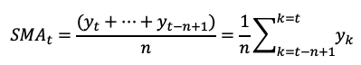
where y1, y2, … are the previous n data points, and n is the number of data points used in the moving average.

An exponential moving average (EMA) is similar to a simple moving average, but it gives more weight to the most recent data points. This means that the EMA is more sensitive to recent changes in the data and responds more quickly to changes in the trend. The formula for an exponential moving average is:

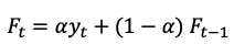
where yt is the current data point, Ft-1 is the previous EMA, and α is a smoothing factor that determines how much weight is given to the most recent data point. The value of α is typically between 0 and 1, with a common choice being α = 0.2.

Often when we inspect a time series plot, we see visible trends and seasonal patterns. The next modeling method decomposes a time series.

Classical univariate seasonal-trend decomposition model

The seasonal-trend decomposition model assumes that the time series can be represented as an additive model of three components:

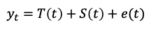
• Trend Component (Tt): This component represents the long-term trend in the time series.
• Seasonal Component (St): This component represents the occurring annual, quarterly, monthly, or weekly fluctuations.
• Irregular Component (et): This component represents the remaining variation in the time series.

Below is an example that the time series is decomposed into trend and seasonality across the sample.

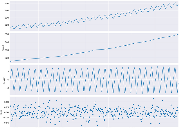
The seasonal-trend decomposition model does not explicitly capture correlations in a sequence. The autoregressive models are designed to capture the sequential patterns.

Autoregressive models to capture sequential patterns

Autoregressive (AR) models capture sequential patterns by modeling the linear relationship between an observation and a fixed number of lagged observations (previous periods). This component is a fundamental part of ARIMA (AutoRegressive Integrated Moving Average) as we have introduced in the previous chapter titled “Automatic ARIMA”.

In an autoregressive model of order p, denoted as AR(p), the value of the time series at any given time t is modeled as a linear combination of its p most recent values. Mathematically, an AR(p) model can be represented as:

By estimating the coefficients b1, b2, …, bp, an autoregressive model captures the sequential dependencies present in the data. These coefficients are typically estimated using methods such as least squares estimation or maximum likelihood estimation.

Autoregression directly models future values as the linear combinations of past values. However, if the values yt are very noisy, autoregression can capture noises as patterns. It may be the case that the observed values, even very noisy, come from underlying values whose trajectory is relatively stable. The Kalman filter provides a new way to consider noisy time series.

Kalman filter to capture latent patterns

The Kalman filter is an algorithm used to estimate the path of a moving object like a car or a plane, based on noisy measurements. It was developed by Rudolf E. Kalman in the 1960s and has since become a widely used tool in various fields, including engineering, robotics, and finance.

Let me use a story to explain the Kalman filter. I live not far from the local beach so sometimes I go there to enjoy my solitude. One late afternoon I was thinking about how to explain the Kalman Filter for my lecture. I saw a seagull flying in the sky and casting a moving shadow on the sparkling ocean. The path of the flying seagull in the sky forms a time series, and the path of shadows is another time series. The path of the shadow on the ocean surface is extremely noisy, though the path in the sky is relatively stable. The positions of the flying seagull in the sky are unreachable and unobservable, but the shadows on the ocean are observable.

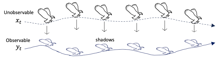
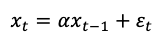
If we use the Kalman filter to model the paths in the sky and on the ocean surface, we can model them with the following equations. First, the unobservable position of the seagull in the sky is Xt, which is a linear combination of the previous location Xt-1 (times a scaler coefficient) and a random white noise:

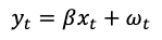
Its shadow on the ocean surface is observable. The shadow position yt is xt times a scaler coefficient plus a white noise.

Kalman filter helps us to consider what we have observed actually coming from latent patterns. The latent patterns are relatively stable but the observables are very noisy. The separation of unobservable and observable patterns helps us not to model the noises as patterns.

State space model to capture latent sequential patterns

The linear assumption of the Kalman filter for the latent variable can be restrictive. In many real-world examples, systems have nonlinear dynamics and measurement functions. State-space models are a general framework for modeling dynamic systems, including both linear and nonlinear systems. In this sense, the Kalman filter is a special case of the state space algorithm.

In a state space model, the observed data is modeled as a function of a set of unobserved latent variables or states, which evolve according to a stochastic process. The observed data is assumed to be a noisy measurement of the true underlying state, and the goal is to estimate the state sequence that best explains the observed data. A state space model can be represented as:

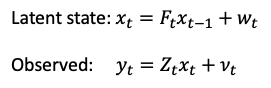
where y(t) is the observed data at time t, x(t) is the latent state at time t, Z(t) is the observation matrix, F(t) is the state transition matrix, v(t) is the observation noise, and w(t) is the process noise.

The above models provide a single-point prediction yt. Real-world applications typically require a range of possible predictions, or prediction intervals, rather than a point estimate. Thus let’s discuss the design for probabilistic predictions.

From point estimates to probabilistic predictions

Probabilistic prediction is the process of estimating the likelihood or probability of a range of outcomes. It is more practical to know the prediction uncertainty rather than provide a single deterministic prediction. For example, is it better just to know “the expected average financial loss is $40M,” or “we have 95% confidence that the financial loss will be between $10M and $70M, with an average of around $40M”? The need for probabilistic forecasts in time series motivates the development of probabilistic predictions.

We can write the latent variables including the state-space models in a general form:

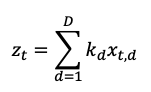
The observed data yt is a function of the latent variable zt plus a white noise term et:

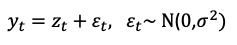
However, we can formulate the observed data yt as drawn from a Gaussian distribution (or other types of distributions). Instead of providing a single range, probabilistic forecasts provide a full probability distribution. Our goal is to find the mean and the standard deviation of the Gaussian distribution. We will maximize the likelihood function like below to find the mean and the standard deviation.

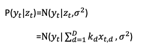
This probabilistic distribution gives us the probabilistic predictions. With the estimated mean and standard deviation, we can provide the probabilistic forecasts. A common approach to representing probabilistic forecasts is through Monte Carlo simulation and quantile forecasts. Quantiles divide the probability distribution into equal parts, such as the median (50th percentile), 90th percentile, or 95th percentile. Each quantile represents a specific level of confidence, allowing decision-makers to assess the range of possible outcomes and their associated probabilities. The next chapter “DeepAR for RNN/LSTM” shows how DeepAR incorporates the probabilistic predictions. It also shows an example of Monte Carlo simulation.

From state space models to multilayer perceptrons (MLPs)

In the state-space models, the relationships between the inputs and outputs are formulated with a clear state structure. However, they can be difficult to apply to complex nonlinear systems. The research community has been thinking of neural network frameworks for time series modeling. In the late 1970s and early 1980s, a new class of models known as Multilayer Perceptrons (MLPs) emerged as an alternative to nonlinear state-space models. Significant academic papers of this line include [2], [3], and [4] by Rosenblatt (1958), Rumelhart, Hinton, (1986), and Hassibi, Stork, Wolff (1993). MLPs use neural network frameworks to model the relationships between the inputs and outputs, thus becoming more flexible and adaptable to a wider range of problems. Today MLP models have been engineered with the availability of deep learning frameworks and libraries like TensorFlow and PyTorch. These frameworks provide high-level APIs, allowing for rapid development and deployment of models.

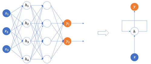
The diagram below shows how an MLP models and predicts the future values yt+1 and yt+2. The MLP is a standard feed-forward neural network with hidden layers in the dashed box. The inputs (the blue dots) are the past values xt-n, …, xt. They also can be any transformations of past values such as moving averages.

Since the state space models can capture the temporal dependencies between the elements in the sequence, MLPs are inspired to incorporate the temporal dependencies. Combining a state-space model with an MLP can be advantageous. The state-space model provides a structured way to model temporal dependencies and uncertainty, while the MLPs offer flexibility in capturing complex patterns and nonlinear relationships in the data. This leads to the invention of the recurrent neural networks.

Recurrent Neural Networks (RNN)

RNNs are called recurrent because they perform the same task for every sample, given the outcome from the previous computations. RNNs maintain a hidden state vector, also called the memory. This hidden state, similar to the ones in state space models, is updated at each time step based on the current input and the previous hidden state. We also can consider RNNs to have a “memory” that passes information from one time step to the next time step.

In RNNs, the same set of parameters (weights) is used at each time step. This allows the network to learn patterns across different time steps and generalize well to sequences of varying lengths.

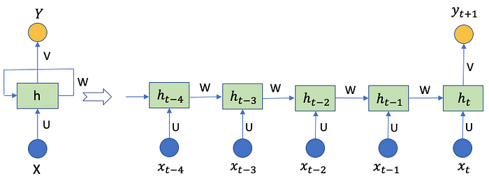
The diagrams below unroll an RNN to a full neural network. The diagram below assumes that memory has five steps. The basic architecture of an RNN consists of a recurrent layer that takes xt-4, xt-3, xt-2, xt-1, and xt, to output a sequence of hidden states ht-4, ht-3, ht-2, ht-1, and ht. The hidden state at time t is computed as a function of the input at time t and the hidden state at the previous time step (t-1): ht = f(ht-1, xt-1).

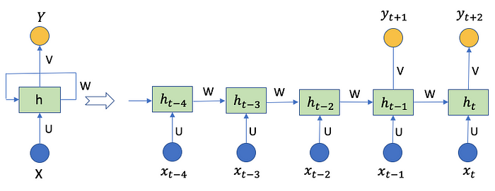
As said in MLPs, the neural network frameworks enable multi-period-ahead predictions. The diagram shows 5 steps xt-4, xt-3, xt-2, xt-1, xt, and two output time steps yt+1 and yt+2.

RNNs are known for the gradient vanishing problem. Let’s see how LSTM and GRU solve the problem.

From RNN to LSTM

An RNN in theory can memorize very long periods through its recurring design. However, the long memories can quickly vanish when training an RNN. This is known as the gradient vanishing problem. The training for an RNN means to compute the first-order derivative, or called the gradient, of the loss function to search for the optimal values. Because RNN is recursive, the first-order derivation process will make a gradient smaller and smaller, then eventually vanish. This mathematical process makes RNN not a good choice to retain memories. We need a recursive structure so that the information does not vanish quickly. This is the motive for LSTM and GRU. (Note: A loss function is a metric that measures the errors between the actual and the predicted values. An optimizer is an algorithm that changes the weights of the neurons to pursue the minimum error. A popular optimizer is the Stochastic Gradient Descent (SGD)).

One of the early breakthroughs in RNNs was the introduction of the Long Short-Term Memory (LSTM) architecture by Hochreiter and Schmidhuber (1997) [5]. The structure is called Long Short-Term Memory because it uses the short-term memory processes to create longer memory. LSTMs solve the gradient vanishing problem by introducing additional gates, input, and forget gates. A gate is a sigmoid function that takes the input at a particular time step and the previous cell state as input and outputs a vector of weights. These gates control the flow of information for what to preserve and what to forget.

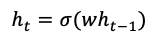
Let’s explore LSTM in great detail. Assume we have a hidden state ℎ𝑡 at time step 𝑡:

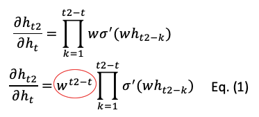
Taking the first-order derivatives we get the following equations. The circled coefficient vector is the key. It will vanish exponentially to zero, or explode exponentially to infinity.

The diagram below shows an LSTM in an RNN framework.

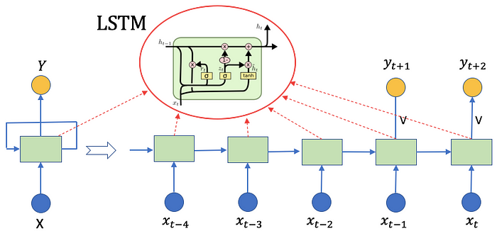
The LSTM has four components: the “input” gates, the forget gates, the cell state, and the output gates to control the information flow.

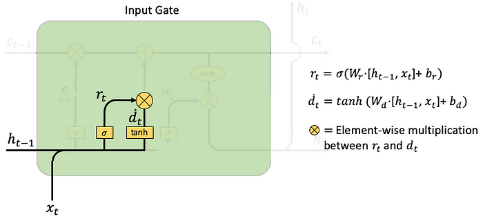
Let’s first highlight the input gate that takes in new information xt. There are two functions to take in new information: rt and dt. The rt concatenates the previous hidden vector ht-1 with the new information xt., i.e., [ht-1, xt], then multiplies with the weight matrix Wr, plus a noise vector br. The dt does something similar. Then rt and dt are multiplied element-wise to get the cell state ct.

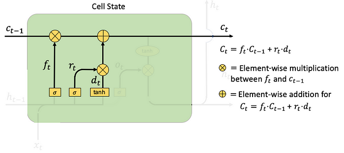
Now let’s highlight the cell state, which includes the forget gate as shown below. The forget gate ft controls the limit up to which a value is retailed in the memory. The cell state calculates an element-wise multiplication between the previous cell state Ct-1 and forget gate ft.

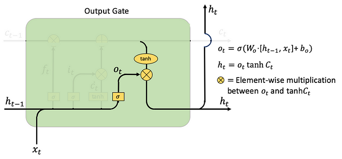
Now let’s highlight the output gate and dim the cell state as the diagram below. The ot is the output gate at time step t, in which the Wo and bo are the weights and bias. The hidden layer ht goes to the next time step. In the final step ht goes up to output as yt.

The vanishing gradient problem can be also resolved by the Gated Recurrent Units (GRUs) introduced by Cho et al. in 2014. Let’s see what it is.

From LSTM to GRU (Gated Recurrent Units)

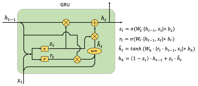
The GRU was invented by Cho et al. (2014) [6]. GRU does not have the cell state and the output gate like those in LSTM and has fewer parameters than LSTM. GRU calls its two gates the reset gate and the update gate. The diagram below shows the full GRU. We will highlight it step by step to explain the reset gate and the update gate.

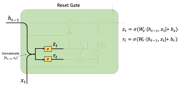
Let’s highlight the reset gate. It does what the input gate and forget gate do in LSTM. It controls how much of the previous hidden state should be ignored when computing the candidate’ hidden state. It also takes into account the previous hidden state and the current input and outputs a reset gate value between 0 and 1. This gate helps the network to reset or forget irrelevant information from the previous hidden state, allowing the network to focus on capturing new patterns and dependencies in the data. It has two gates in sigmoid functions. The gate rt determines if the previous hidden state should be ignored. The gate zt is generated for the update gate. (The notations Wz and Wr are the weight parameters to be trained, bz and br are the noise vectors.)

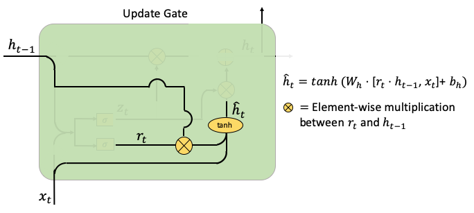
Let’s highlight the update gate. The update gate in a GRU determines how much of the previous hidden state should be retained and how much of the new candidate’ hidden state should be incorporated. It takes into account the previous hidden state and the current input, then outputs an update gate value between 0 and 1. This gate allows the network to selectively update the hidden state, preventing the vanishing gradient problem by allowing relevant information to flow through.

First, let’s talk about rt and ht-1 as shown below. The multiplication means how much of ht-1 will be retained or ignored. This creates a temporal hat(ht) to be used for the update of ht. (The Wh and bh are weight parameters and the noise vectors.)

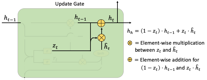
Second, the update gate computes the weighted average between ht-1 and hat(ht). The weight is zt. If zt is close to zero, the past information contributes little and new information contributes more.

Conclusions

In this chapter, we learned the reasons for a new time series model to solve the challenges. We have surveyed the history of time series modeling from the simple moving average, seasonal-trend decomposition, ARIMA, Kalman filter, and state space model. We also learned MLPs, and then RNN/LSTM/GRU. We have learned the design for probabilistic predictions.

In the next chapter, we will learn the DeepAR framework, which is based on RNN/LSTM. We will use the GluonTS library to provide multiple forecasts, and multiple time series, and provide the prediction uncertainty.

References

• [1] G. W. Morrison and D. H. Pike, “Kalman filtering applied to statistical forecasting,” Manage. Sci., vol. 23, no. 7, pp. 768–774, 1977.
• [2] Rosenblatt, F. (1958). The perceptron: a probabilistic model for information storage and organization in the brain. Psychological review, 65 6, 386–408
• [3] Rumelhart, D.E., Hinton, G.E., & Williams, R.J. (1986). Learning internal representations by error propagation.
• [4] Hassibi, B., Stork, D.G., & Wolff, G.J. (1993). Optimal Brain Surgeon and general network pruning. IEEE International Conference on Neural Networks, 293–299 vol.1.
• [5] Hochreiter, S., & Schmidhuber, J. (1997). Long short-term memory. Neural Computation, 9(8), 1735–1780. https://doi.org/10.1162/neco.1997.9.8.1735
• [6] Cho, K., van Merrienboer, B., Gulcehre, C., Bougares, F., Schwenk, H., & Bengio, Y. (2014). Learning phrase representations using RNN encoder-decoder for statistical machine translation. In Conference on Empirical Methods in Natural Language Processing (EMNLP 2014)