Summary

This context describes a use case application of Amazon's DeepAR for stock price forecasts using multiple stock price series and explains the process of installing and using gluonts for this purpose.

Abstract

The context begins by introducing Amazon's DeepAR, a global model that is suitable for multi-step forecasts, multi-series forecasts, and can provide forecasts with uncertainty. The author then explains the use case application of DeepAR for stock price forecasts, which are driven by economic indicators, market sentiment, or news and events. The post provides links to related posts on algorithmic trading and reinforcement learning for algorithmic trading. The author then provides code for installing gluonts and selecting daily prices of large-cap stocks from 2020 to 2024. The post also includes code for plotting the stock prices and splitting the time series into training and test data. The author explains the need to convert the dataset to a gluonts compatible data format and provides code for doing so. The post then provides code for modeling the data using DeepAREstimator() function and explains the parameters used. The author also explains the need to make forecasts and provides code for doing so using make_evaluation_predictions() function. Finally, the post provides code for visualizing the predictions and generating evaluation metrics.

Bullet points

DeepAR is a global model that is suitable for multi-step forecasts, multi-series forecasts, and can provide forecasts with uncertainty.
Stock prices tend to follow a set of common volatility factors driven by economic indicators, market sentiment, or news and events.
The post provides links to related posts on algorithmic trading and reinforcement learning for algorithmic trading.
The author provides code for installing gluonts and selecting daily prices of large-cap stocks from 2020 to 2024.
The post includes code for plotting the stock prices and splitting the time series into training and test data.
The author explains the need to convert the dataset to a gluonts compatible data format and provides code for doing so.
The post provides code for modeling the data using DeepAREstimator() function and explains the parameters used.
The author explains the need to make forecasts and provides code for doing so using make_evaluation_predictions() function.
The post provides code for visualizing the predictions and generating evaluation metrics.

Application: Amazon’s DeepAR for Stock Forecasts

In “DeepAR for RNN/LSTM”, we have learned that DeepAR builds a global model and is suitable for multi-step forecasts, multi-series forecasts, and can provide forecasts with uncertainty. We have tested its predictability of DeepAR with the multiple time series of Walmart store weekly sales. Much of the explanations were provided in “DeepAR for RNN/LSTM” and “The History of Time Series Modeling Techniques”, you are encouraged to read them if you have not.

This post is a short use case application. Let’s experiment DeepAR with multiple stock price series. Stock prices tend to follow a set of common volatility factors driven by economic indicators, market sentiment, or news and events. A global model of DeepAR seems suitable for the multi-series forecasts. We are also interested in the forecasts of multiple periods. The forecasts help identify long-term trends and patterns in stock prices for sophisticated trading strategies, such as trend following, mean reversion, or momentum trading. Further, we are interested in the probabilistic uncertainty that DeepAR can provide for risk management. The interest for the stock price application is renewed by more advanced techniques. They offer new ways to advance in the prediction accuracy as well as trading strategies. You may reference everal recent related posts:

First, let’s install gluonts.

# Installation of gluonTS
!pip uninstall numpy # Downgrade numpy to 1.23
!pip3 install mxnet-mkl==1.6.0 numpy==1.23.1
!pip install gluonts==0.14.2
!pip install yfinance

For this study, we select the daily prices of the following large-cap stocks from 2020 to 2024.

import yfinance as yf
data = yf.download(["SPY","MSFT","AMZN","GOOG","PGR"], start="2020-01-01", end="2024-12-31")
data = data[[('Adj Close', 'AMZN'),('Adj Close', 'GOOG'),('Adj Close', 'MSFT'),('Adj Close',  'PGR'),('Adj Close',  'SPY')]]
data.columns = ['AMZN','GOOG','MSFT','PGR','SPY']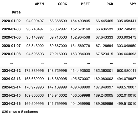

Let’s plot them to observe their movements.

%matplotlib inline
import pandas as pd
import numpy as np
from matplotlib import pyplot as plt

data.plot(figsize=(12, 4))
plt.legend(loc='upper left')
plt.title("Stocks")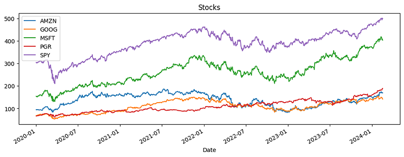

We then split the give time series into the training and test data. We will take 85% of the data as the “in-time” training data, and the rest 15% as the “out-of-time” test data.

print("The time series has", data.shape[0], "data points")
len_train = int(data.shape[0] * 0.85)
train_data = data[0:len_train]
test_data = data[len_train:]
[train_data.shape, test_data.shape]

The time series has 1039 data points. (883,5) and (156,5).

Any time series data should have three basic elements: the start date, the target data, and the frequency of the data. The data format of GluonTS expects these three basic elements. In the following code, we will convert our dataset to a gluonTS compatible data format. The code gets the start date by computing the minimum date, and the columns as the targets.

# Prepare the data for deepAR format
from gluonts.dataset.common import ListDataset
from gluonts.dataset.field_names import FieldName

def to_deepar_format(dataframe, freq):
    start_index = dataframe.index.min()
    data = [{
                FieldName.START:  start_index,
                FieldName.TARGET:  dataframe[c].values,
            }
            for c in dataframe.columns]
    print(data[0])
    return ListDataset(data, freq=freq)
train_data_lds = to_deepar_format(train_data, 'D')
test_data_lds = to_deepar_format(test_data, 'D')

The modeling code has quite succinct lines. The code below uses the DeepAREstimator() function and I will explain accordingly.

# api: https://ts.gluon.ai/stable/api/gluonts/gluonts.mx.model.deepar.html
# paper: Salinas, David, Valentin Flunkert, and Jan Gasthaus. “DeepAR: Probabilistic forecasting with autoregressive recurrent networks.” arXiv preprint arXiv:1704.04110 (2017).

from gluonts.mx.model.deepar import DeepAREstimator
#from gluonts.torch.model.deepar.estimator import DeepAREstimator
from gluonts.mx.trainer import Trainer

prediction_length = 30
context_length = 30
num_cells = 100
num_layers = 8
epochs= 150
freq="D" # Our data is daily

estimator =   DeepAREstimator(freq=freq,
                                context_length=context_length,
                                prediction_length=prediction_length,
                                num_layers=num_layers,
                                num_cells=num_cells,
                                cardinality=[1],
                                trainer=Trainer(epochs=epochs))
predictor = estimator.train(train_data_lds)

Once the modeling task completes, let’s make the forecasts. When validating a time series model, we conduct forecasts within the out-of-time or test window and utilize the test dataset to assess the forecasting performance. This procedure is conveniently encapsulated within the ‘make_evaluation_prediction’ function. This function predicts the last window of the test data and evaluates the model’s performance accordingly. It first extracts the final window of length ‘prediction_length’ from the test data. Then it uses the remaining test data to generate predictions. Then it compares the predictions against the actual values within the final window of length ‘prediction_length’.”

from gluonts.evaluation.backtest import make_evaluation_predictions
forecast_it, ts_it = make_evaluation_predictions(
    dataset=test_data_lds,
    predictor=predictor,
)
tss = list(ts_it)
forecasts = list(forecast_it)

Further, we need to provide the probabilistic forecasts. GluonTS generates probabilistic forecasts using probability distributions to capture the uncertainty inherent in future predictions, enabling users to quantify the potential range of outcomes. The default distribution in GluonTS for Monte Carlo simulation is Gaussian Distribution. GluonTS estimates the mean (μ) and standard deviation (σ) of the Gaussian distribution, where the former signifies the point forecast while the latter indicates the level of uncertainty surrounding the prediction. GluonTS can employ other probability distributions such as Student’s t-Distribution, Negative Binomial Distribution, and Gamma Distribution.

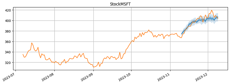
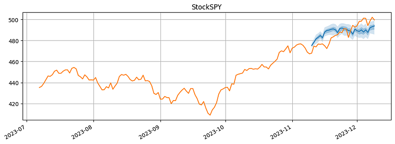
Let’s visualize the predictions.

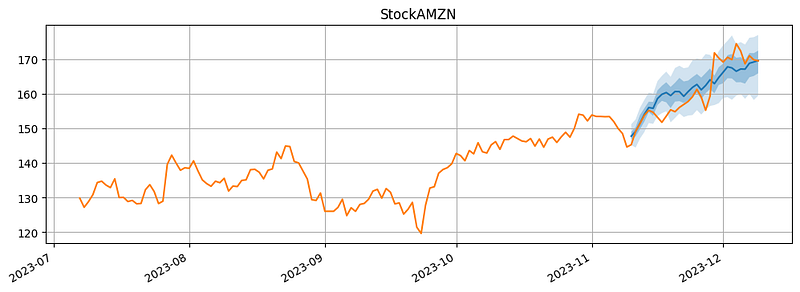
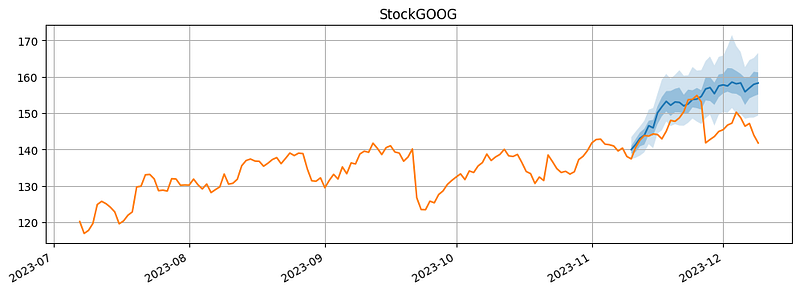
for k in range(len(forecasts)):
  fig, ax1 = plt.subplots(1, 1, figsize=(12, 4))
  forecasts[k].plot(ax = ax1)
  tss[k].plot(ax = ax1)
  ax1.get_legend().remove()
  plt.grid(which="both")
  plt.title("Stock" + data.columns[k])
  plt.show()

The predictions are generally consist with the actual values. Although the prediction outcomes are promising, we still need to scrutinize the predictions since stock market prices are always volatile.

The following code produces the evaluation metrics. Here we do not output the metrics just to save space.

from gluonts.evaluation import Evaluator

evaluator = Evaluator()
agg_metrics, item_metrics = evaluator(iter(tss), iter(forecasts), num_series=len(test_data_lds))

import json
print(json.dumps(agg_metrics, indent=4))

The Python notebook is available via this link.