A Tutorial on Multi-step Time Series Forecasts

Two primary strategies for multi-step forecasts

The human pursuit of forecasting has never ceased, from the ancient sages peering into celestial patterns to the cutting-edge algorithms of today. The quests have legitimate reasons. We need the weather forecasts for a week, not just the next hour, to plan trips. A manufacturer needs forecasts for several months but not a forecast for the next hour. We need to plan for the near future and coordinate with others. We forecast the near future although we are aware of the challenges in forecasting.

From a data science technical perspective, there is a big difference between forecasting one period and multiple periods, and the latter is harder. Forecasting multiple periods demands a comprehensive understanding of long-term patterns and dependencies. It is proactive and requires models to capture the intricate dynamics over time. Knowing there are distinct challenges in multi-step forecasting, you will understand why I set this topic as a standalone topic. In the forecasting literature, there are already voluminous papers that fill the gap between the “one-step” forecast and “multi-step” forecasts. This is a good news.

Let me assume we need to start from scratch and do not know the past literature. How do we even think of the strategies for multi-step forecasting? Maybe let’s start with the one-step forecasting models like ARIMA. How do we make it multi-step? Maybe one way is to use the same model recursively. We get the one-period prediction from the model as the input to forecast the next period. Then we take the prediction for the second period as the input to forecast the third period. We can iterate through all the periods by using the predictions of the prior periods. This is exactly what the recursive forecasting or iterative forecasting strategy does.

What else can we do? We have learned to formulate a univariate time series as a tree-based modeling problem in “A Tutorial on Tree-based Time Series Forecasting”. We can model the value of one period, either the current period y(t) or any future period y(t+n), as the target of a tree-based model. The model will produce an unbiased value for one period. What if we build n models that each produce the forecast for the nth period? Then all we need to do is to combine the forecasts of the n models. This is exactly the direct forecasting strategy. Although it sounds cumbersome, it has produced proven results. Part of the reason for its success is because tree-based models for a single target are usually effective and different models can capture the intricate dynamics over time. There are a few other alternative strategies but mainly the derivations of these two approaches. That’s why I consider the two approaches as the main strategies. Let’s re-cap. The two primary strategies are:

Recursive forecasting
Direct forecasting for n periods

These two approaches involve cumbersome data re-structuring and model iterations. The recursive strategy has been coded in the classical Python library “statsmodels” as explained in its forecasting procedure. I will use the open-source Python library “Sktime” library that makes both the recursive and the direct forecasting methods easy. Sktime wraps up a wide range of tools including “statsmodels” under a unified API for time series forecasting, classification, clustering, and anomaly detection (Markus et al. (2019, 2020)).

In this post, I will walk you through how to think about the strategies to produce multi-step forecasts, the code for multi-step forecasts, and the evaluations. Specifically, we will do:

The recursive strategy for multi-step forecasts
The direct forecasting strategy for n periods with n models
The recursive strategy with ARIMA

The Python notebook is here for download. First, let’s take care of the software requirement.

Installation of software

We will install the sktime library and the lightGBM library from PyPi.

!pip install sktime
!pip install lightgbm

Recursive forecasting

As said before, the recursive strategy for multi-step forecasts involves making predictions for one step ahead, and then using those predictions as inputs to forecast future time steps iteratively. In this process, there is only one model. The model generates a forecast then is fed with the forecast to generate the next forecast and so on. Let’s write it down in a step-by-step process:

Modeling: Train a time series forecasting model using the training data to predict a one-step-ahead prediction. This model could be a traditional time series model like ARIMA, an exponential smoothing model, or a machine learning model such as lightGBM (as shown in this chapter).
Generating the 1st prediction: Use the trained model to predict the next time step based on the available historical data.
Feeding the predicted value as the input data to the model for the next prediction: This means appending the predicted value to the historical data, creating an updated time series.
Forecasting iteratively: Repeat the process iteratively by using the updated time series as input to the model for each subsequent step. In each iteration, the model takes into account the previously predicted values, making multi-step forecasts. Continue the iterative forecasting process until you reach the number of steps into the future you want to predict.

What could be the downsides? One perceivable issue is the degradation in prediction accuracy over a long horizon. The forecasting errors in prior predictions can accumulate in latter forecasts. As long as the model is complex enough to capture the intricate patterns, this may be acceptable.

This modeling strategy appears sound. I will use Google Colab and load the electric consumption data. Let me skip the data description, which has been explained in “A Tutorial on Tree-based Time Series Forecasting”.

%matplotlib inline
from matplotlib import pyplot as plt
import pandas as pd
import numpy as np

from google.colab import drive
drive.mount('/content/gdrive')

path = '/content/gdrive/My Drive/data/time_series'
data = pd.read_csv(path + '/electric_consumption.csv', index_col='Date')
data.index = pd.to_datetime(data.index)
data = data.sort_index() # Make sure the data are sorted
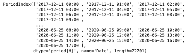
data.index = pd.PeriodIndex(data.index, freq='H') # Make sure the Index is sktime format
data.index

The only thing I want to point out is the use of pd.PeriodIndex() to make the index conforms to the sktime format.

Below we take a series from the Pandas data frame. The Pandas Series keeps the index that is required by sktime.

y = data['Consumption']
y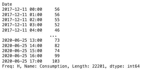

We are about to apply the recursive forecasting approach. Let’s build a lightGBM model with the same hyper-parameters as those in “A Tutorial on Tree-based Time Series Forecasting”. In the Python Notebook, I also demoed a GBM model (not shown here) and you can experiment with other models.

import lightgbm as lgb
lgb_regressor = lgb.LGBMRegressor(num_leaves = 10,
              learning_rate = 0.02,
              feature_fraction = 0.8,
              max_depth = 5,
              verbose = 0,
              num_boost_round = 15000,
              nthread = -1
)
lgb_forecaster = make_reduction(lgb_regressor, window_length=30, strategy="recursive")
lgb_forecaster.fit(train)

Notice we just specify “recursive” as the value for the strategy hyperparameter. Later when we do the direct forecasting approach, we will enter “direct”. It is quite easy, isn’t it? I will explain make_reduction() in the end.

Next, we need to generate a list of future periods in numbers. I set 100 periods for the future horizon (fh), which is [1,2,…, 100]. Then I generate the forecasts for the 100 periods. Later in the direct forecasting section I will also use 100 periods so we can compare the results.

vlen = 100
fh = list(range(1, vlen,1))
y_test_pred = lgb_forecaster.predict(fh= fh)
y_test_pred

How do the forecasts perform when compared with the actual values in the testing data? Let’s match the 100 periods of the actual values and the forecasts and plot them.

from sktime.utils.plotting import plot_series
actual = test[test.index<=y_test_pred.index.max()]
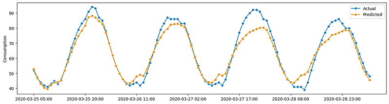
plot_series(actual, y_test_pred, labels=['Actual', 'Predicted'])
plt.show()

I use the function plot_series() which is just a wrapper of a matplotlib function. The results look satisfactory:

Figure (A): Recursive strategy with lightGBM

Two common evaluation metrics are mean absolute percentage error (MAPE) and symmetric MAPE. Again, sktime makes it easy by turning the hyperparameter “symmetric” on and off:

from sktime.performance_metrics.forecasting import mean_absolute_percentage_error
print('%.16f' % mean_absolute_percentage_error(actual, y_test_pred, symmetric=False))
print('%.16f' % mean_absolute_percentage_error(actual, y_test_pred, symmetric=True))

The outcomes are as follows. Later we will compare these two numbers with those in the direct forecasting approach.

MAPE: 0.0546382493115653
sMAPE: 0.0547477326419614

Great. We have successfully built multi-forecasts using the recursive method. Next, let’s learn the direct forecasting strategy.

Direct forecasting for n periods

Knowing the recursive forecasting strategy, let’s consider the direct forecasting strategy. We will build many individual models. Each model is responsible for predicting a specific future period. Although building many models can be time-consuming, it is nevertheless machine time not my brain time. I do enjoy a coffee break while exploiting CPU power (CPU is enough). Let’s write down the process step by step:

Model Training: Train separate models for each of the future time steps. For example, if you want to predict the next 100 periods, train 100 separate models, each responsible for predicting the value at its respective time step.
Forecasting: Use each trained model to independently generate its forecast for its specific time. These models can operate in parallel because their predictions are not dependent on each other.
Combining Forecasts: Just concatenate the forecasts.

One advantage of this direct forecasting strategy is its ability to capture the specific patterns in each forecasting horizon. Each model can be optimized for the time step it is responsible for, potentially leading to improved accuracy.

Let’s do it. We will build the same lightGBM as the regressor and use make_reduction(). The only difference is “direct” instead of “recursive” as the hyperparameter. Very easy, isn’t it?

from sktime.forecasting.compose import make_reduction
import lightgbm as lgb
lgb_regressor = lgb.LGBMRegressor(num_leaves = 10,
              learning_rate = 0.02,
              feature_fraction = 0.8,
              max_depth = 5,
              verbose = 0,
              num_boost_round = 15000,
              nthread = -1
)
lgb_forecaster = make_reduction(lgb_regressor, window_length=30, strategy="direct")

We will generate a list of 100 periods [1,2,…, 100] as the forecasting horizon (fh). This will build 100 lightGBMs that each forecasts one of the 100 periods. Building 100 lightGBMs can be time-consuming, that’s why I only demo 100 periods. Feel free to take a coffee break.

vlen = 100
fh=list(range(1, vlen,1))
lgb_forecaster.fit(train, fh = fh)

After your coffee break, let’s generate the forecasts:

y_test_pred = lgb_forecaster.predict(fh=fh)
y_test_pred

Great. We will plot the actual values in the testing data against our forecasts.

from sktime.utils.plotting import plot_series
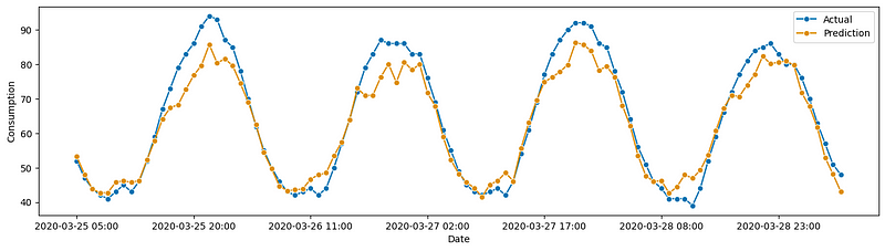
plot_series(actual, y_test_pred, labels=["Actual", "Prediction"], x_label='Date', y_label='Consumption');

The forecasts appear satisfactory. Remember this is because each forecast comes from a separate model with its own features.

Figure (B): Direct forecasting strategy with lightGBM

Finally, let’s review the evaluation metrices:

from sktime.performance_metrics.forecasting import mean_absolute_percentage_error
print('%.16f' % mean_absolute_percentage_error(actual, y_test_pred, symmetric=False))

print('%.16f' % mean_absolute_percentage_error(actual, y_test_pred, symmetric=True))

The MAPE and sMAPE are very close to those by the recursive method. We will feel comfortable in using either strategy in our case.

MAPE: 0.0556899099509884
sMAPE: 0.0564747643400997

We have seen the above handy work by make_reductoin(). I guess you become curious about it. Let’s explore more about it.

What does make_reduction() do?

The above lightGBM model is a supervised learning model. Any supervised learning models need data frames that have x and y for model training. How does make_reduction() turn a univariate time series into a data frame?

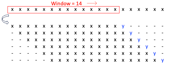
The make_reduction() function does a lot of work. The two primary parameters are strategy for ‘recursive’ or ‘direct’, and window_length for the length of a sliding window. The sliding window moves alone with the univariate time series to create samples. The values in the sliding window are the x values.

I will explain the recursive and the direct strategies below. Let me assume there are 20 points and a length of 14 for the window.

Recursive strategy

When the strategy is the recursive forecasting strategy, the value in front of the sliding window is the target value. Figure (D) slides the window of 14 and generates a data frame of 6 samples. The target values are the y values in blue color. This data frame is used to train the model.

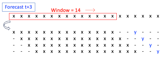
Direct forecasting strategy

The direct forecasting strategy builds a model for each of the future target periods. Assume the target is the value in t+3. Figure (D) slides the window of 14 and generates a data frame of 4 samples. The target values are the y values in t+3. This data frame is used to train the model that predicts the y value of t+3.

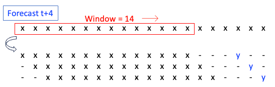
Figure (E): Make_reduction() for the direct strategy for y_t+3

Assume the target is the value in t+4. Figure (D) slides the window of 14 and generates a data frame of 3 samples. The target values are the y values in t+4. This data frame is used to train the model which is to predict the y value of t+4.

Figure (F): Make_reduction() for the direct strategy for y_t+4

Multi-step forecasts with ARIMA

It will be valuable to understand how Sktime does ARIMA and provide its multi-step forecasts. Remember that Sktime wraps the Python library “pmdarima”, a popular ARIMA library that can do multi-step forecasts. So Sktime does not do the multi-step forecasts but the “pmdarima” library does. Once the ARIMA model is built, it still makes one-step-ahead predictions for each time point in the forecast horizon. Then it applies the recursive strategy by generating predictions iteratively. The predicted value for the next time point is used as an input for predicting the subsequent time point. You will need to install “pmdarima.”

!pip install pmdarima

Let me demonstrate the function temporal_train_test_split() to split the data into training and test data.

from sktime.forecasting.model_selection import temporal_train_test_split
train, test = temporal_train_test_split(y, train_size = 0.9)

The following code builds the model and provides the forecasts. Notice the code does not use the make_reduction() function of Sktime. This is because the multi-step forecasts are provided by the AutoARIMA model. I am not going to show the outputs. You can find them in the Python notebook.

from sktime.forecasting.arima import AutoARIMA

arima_model = AutoARIMA(sp=12, suppress_warnings=True)
arima_model.fit(train)

# Future horizon
vlen = 100
fh=list(range(1, vlen,1))

# Predictions
pred = arima_model.predict(fh)
from sktime.performance_metrics.forecasting import mean_absolute_percentage_error
print('%.16f' % mean_absolute_percentage_error(test, pred, symmetric=False))

Knowing the make_reudction function of Sktime, I guess you also want to know Sktime. Before we end this chapter, let’s briefly review Sktime.

A brief introduction to Sktime

The Python library Sktime is an open-source library that combines many forecasting tools under a unified API (Markus et al. (2019, 2020)). It wraps up a wide range of tools and algorithms for time series forecasting, classification, clustering, and anomaly detection. Some key features include:

Time series data preprocessing: This includes missing values handling, imputing, and transformation.
Time series forecasting: It includes common time series modeling algorithms that I list in the next paragraph.
Time series classification and clustering: It includes classification models like time series k-nearest neighbors (k-NN) and clustering models like time series k-means.
Time series annotation: It allows for labeling and annotating time series data, which is useful for tasks like anomaly detection and event detection.

Sktime includes Exponential Smoothing (ES), the classical Autoregressive Integrated Moving Average (ARIMA) and Seasonal ARIMA (SARIMA) models. It covers structural models like Vector Auto-regression (VAR), Vector Error Correction Model (VECM), Structural Time Series (STS) models. It can do neural network models including Time Convolutional Neural Network (CNN), Fully Connected Neural Network (FCN), Long Short-Term Memory Fully Convolutional Network (LSTM-FCN), Multi-scale Attention Convolutional Neural Network (MACNN), Time Recurrent Neural Network (RNN), Time Convolutional Neural Network (CNN). I am interested in other libraries that it has wrapped in. Here let’s take a look:

From “statsmodels”: Holt-Winter’s Exponential Smoothing, Theta Forecaster, and ETS. The ETS model is the decomposition model for trend (T), seasonal (S), and an error term (E).
From “pmdarima”: ARIMA and AutoARIMA
From “tbats”: TBATS stands for Trigonometric seasonality, Box-Cox transformation, ARMA errors, Trend and Seasonal components.
From “Prophet”: the Prophet forecaster

Conclusions

In this chapter, we’ve learned how to think of the modeling strategies from one-period forecasting to multiple periods. We learned the two primary approaches: recursive forecasting and direct forecasting for n period. We learned the Python package “sktime” which let us perform the two strategies easily. Although we demonstrated the lightGBM model, we can use any other models such as ARIMA, linear regression, GBM, or XGB as the regressors.

References

- Markus Löning, Anthony Bagnall, Sajaysurya Ganesh, Viktor Kazakov, Jason Lines, Franz Király (2019): “sktime: A Unified Interface for Machine Learning with Time Series”
- Markus Löning, Tony Bagnall, Sajaysurya Ganesh, George Oastler, Jason Lines, ViktorKaz, …, Aadesh Deshmukh (2020). sktime/sktime. Zenodo. http://doi.org/10.5281/zenodo.3749000