A Tutorial on Tree-based Time Series Forecasting

In around 2020s, there were a series of prize competitions for time series forecasting called the M competition, hosted by the International Institute of Forecasters and its affiliation with the prestigious journal, the International Journal of Forecasting. The winning models were awarded with prizes from $25,000 to $2,000. The competitions have drawn researchers from the world to invent new time series models.

Who were the winners? Surprisingly, the top ranking models were dominated by tree-based machine learning methods. In particular, gradient-boosting models like LightGBM (Ke et al., 2017) prevailed the competitions, as documented in Januschowski et al., 2022. It is for this important reason that I include the tree-based time series forecasting in this book. Although I’ve introduced handy tools like Prophet and NeuralProphet, it is extremely valuable to understand tree-based models.

Now we venture into a new territory that is different from the classical ARIMA-style time series modeling. We know that a supervised learning model requires a target variable and features, yet a univariate time series seems to have limited information. Is it enough to generate many features for a supervised learning models? A straightforward way is to create a lot of lagged variables. Further, let’s talk about the target. We are using the past terms to predict the future terms, right? Is it only one-step-ahead or will be multi-step-ahead? It is just for these important reasons that there have been many successful models by academic researchers and practitioners.

In this post, we will do the fundamental steps:

Creating features from a univariate time series
Supervised learning framework for one-step-ahead forecast
Building lightGBM forecasting models
Providing model explainability

These fundamental steps will prepare you to do the multi-step forecasting. We just focus on lightGBM, but the procedure applies to other regressors like Random Forest (RF) or Gradient Boosting Machine (GBM) or Extreme Gradient Boosting (XGB). The Python Notebook is available here for you to download.

In case you have not seen NeuralProphet, you can click here:

First, let’s take care of the software requirement.

Installation of software

We will install the lightGBM library by pip install lightgbm from PyPi.

Creating features from a univariate time series

It seems we only have limited information in a univariate time series that has has dates and values. In ARIMA modeling we have learned it uses past values to forecast the future values using its past values, so the past values must be important candidates to be the features. This affords to create many lagged regressors such as yt-1, yt-2, …, to yt-n. What else can we do?

Actually the time index is a valuable field and we can create features. I checked quotes about time and a few quotes already imply feature engineering: “Time is a fingerprint, leaving its mark on special moments.” “Time is a great teacher.” True, there are annual events repeating in our lives. The calendar events mark our lives in the past and teach us for the future. So why don’t we start with time-related features?

Create time-based features

Today is January 19, 2024 as I am writing this chapter. It is (i) the first month, (ii) the 19th day of the month, (iii) the first quarter, and (iv) it is Friday in 2024. I can easily create four features and I can think of more calendar-features. In fact, we do not need to re-invent the wheel because the pandas series “date” class already has a long list of features. Below I just choose some common functions to create features.

def create_date_features(df):
    df['month'] = df.date.dt.month
    df['day_of_month'] = df.date.dt.day
    df['day_of_year'] = df.date.dt.dayofyear
    df['week_of_year'] = df.date.dt.weekofyear
    df['day_of_week'] = df.date.dt.dayofweek + 1
    df['year'] = df.date.dt.year
    df['quarter'] = df.date.dt.quarter
    df['hour_of_day'] = df.date.dt.hour
    df['weekday'] = df.date.dt.weekday
    df['is_year_start'] = df.date.dt.is_year_start.astype(int)
    df['is_year_end'] = df.date.dt.is_year_end.astype(int)
    df['is_month_start'] = df.date.dt.is_month_start.astype(int)
    df['is_month_end'] = df.date.dt.is_month_end.astype(int)
    df['is_quarter_start'] = df.date.dt.is_quarter_start.astype(int)
    df['is_quarter_end'] = df.date.dt.is_quarter_end.astype(int)
    df['is_quarter_end'] = df.date.dt.is_quarter_end.astype(int)
    return df
df = create_date_features(df)
df.head()

Great. Let’s bring in real data. I will use a dataset in Kaggle. You will need to download the dataset from Kaggle to your local computer or Google Colab (if you are not using Kaggle as your platform).

%matplotlib inline
from matplotlib import pyplot as plt
import pandas as pd
import numpy as np

# Use google colab
from google.colab import drive
drive.mount('/content/gdrive')

# Use the electric consumption dataset
path = '/content/gdrive/My Drive/data/time_series'
data = pd.read_csv(path + '/electric_consumption.csv')
data.tail()

This dataset has the hourly records for the electricity consumption from 2017 to 2020. In addition to the fields “Date” and “Consumption”, it also has other fields:

data.columns
Index(['Date', 'Homestead_maxtempC', 'Homestead_mintempC',
       'Homestead_DewPointC', 'Homestead_FeelsLikeC', 'Homestead_HeatIndexC',
       'Homestead_WindChillC', 'Homestead_WindGustKmph',
       'Homestead_cloudcover', 'Homestead_humidity', 'Homestead_precipMM',
       'Homestead_pressure', 'Homestead_tempC', 'Homestead_visibility',
       'Homestead_winddirDegree', 'Homestead_windspeedKmph', 'Consumption'],
      dtype='object')

We will just use the “Date” and “Consumption” fields for our univariate time series.

df = data[['Date','Consumption']].copy() # Only the two fields
df.columns = ['date','y'] # Rename the target to be 'y' for easy coding
df["date"] = pd.to_datetime(df["date"]) # Convert to pandas datetime format
df = df.sort_values(by='date') # Make sure it is sorted by date
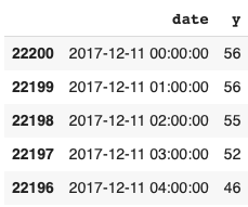
df.head()

The first few records are:

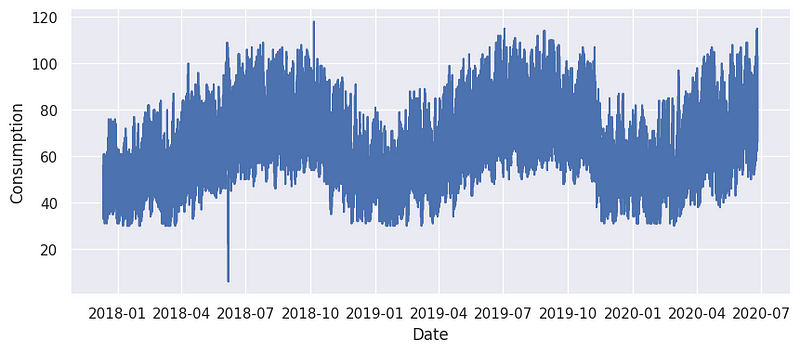
We can plot it:

plt.figure(figsize=(10,4))
plt.plot(df['date'], df["y"])
plt.xlabel("Date")
plt.ylabel("Consumption")
plt.show()

The obvious patterns are cyclical patterns.

Great. Let’s apply our function to create date features:

df = create_date_features(df)
df.head()

The following fields are easily created.

There is one more step we need to do. A few fields should not be used as numerical features but categorical in our models. We will turn them into dummy variables:

to_dummy = ['weekday', 'month', 'quarter', 'year', 'day_of_month', 'week_of_year', 'day_of_week', 'hour_of_day']
df = pd.get_dummies(df, columns= to_dummy)

Great. Up to now we have create a list of features. Let’s learn how to create lagged variables.

Create lagged and future features

You may have already known that the regressors in auto-regressive model are just lagged values. We can use .shift(n) to create lagged features. Below I create three lagged features in a different dataset ff.

ff = df.copy()
ff['y-1'] = ff['y'].shift(1)
ff['y-2'] = ff['y'].shift(2)
ff['y-3'] = ff['y'].shift(3)
ff.head()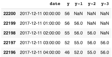

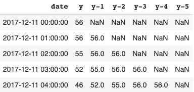
We can write a forloop to create multiple lagged features. Below I will create 5 lagged variables in a different dataset ff:

ff = df.copy()

def create_lagged(df, n_vars):
  # Use a forloop
  for i in range(n_vars):
    # The name will be y-1, y-2, etc.
    name = ('y-%d' % (i+1))
    df[name] = df['y'].shift(i+1)
  return df

ff = create_lagged(ff, 5)
ff.head()

The outputs are:

Obviously, we can also shift the values forward to become future target values as shown in the following demo dataset ff.

ff = df.copy()
ff['y+1'] = ff['y'].shift(-1)
ff['y+2'] = ff['y'].shift(-2)
ff['y+3'] = ff['y'].shift(-3)
ff.tail()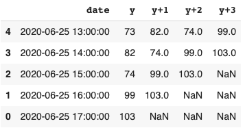

Okay. Let’s formally create 25 lagged variables to the modeling data df for modeling.

df = create_lagged(df, 25)
df.columns

The df dataset will have [‘date’, ‘y’, ‘y-1’, …, ‘y-25’].

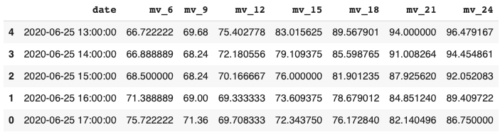
Is that all? No, the story just begins. Since we have the past values, we can create a whole host of summary statistics like the sum or average in the past n hours, days, or weeks. Below I just create the moving averages.

Creating moving averages

We can create the moving averages for the past 6, 9, 12, 18, 21, and 24 hours.

def roll_mean_features(df, windows):
    df = df.copy()
    for window in windows:
        df['mv_' + str(window)] = df['y'].transform(
            lambda x: x.shift(1).rolling(window=window, min_periods=10, win_type="triang").mean())
    return df
df = roll_mean_features(df, [6, 9, 12, 15, 18, 21, 24])
df.tail()

The outputs look like this:

Supervised learning framework for one-step-ahead forecast

Let’s re-cap what we will do in the supervised learning modeling. The target variable is y. The features are the lagged terms y-1, …, y-25, as well as the time-related variables and the moving average variables.

y = fn(yt-1, yt-2, …, yt-25, … )

It says for given yt-1 to yt-25, the model can produce the next period yt. In other words, this model will produce a one-step-ahead forecast.

This is an important area of studies. In many real-world applications we are often interested in multi-step forecasts. What if we want to predict multiple-step-ahead? The conventional approach is to build n models to forecast next n periods.

y+1 = fn_1(yt-1, yt-2, …, yt-25, … )

y+n = fn_n(yt-1, yt-2, …, yt-25, … )

Then we concatenate the y, y+1, … y+n forecasts. In next post, I will introduce more approaches for multi-step forecasts. Let’s now just focus on a model that produces the one-step-ahead forecast.

Building lightGBM forecasting models

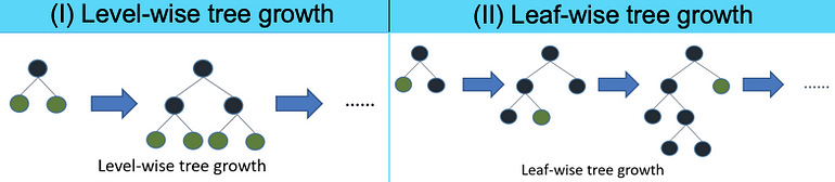
LightGBM is a gradient boosting framework developed by Microsoft. It also provides better accuracy by using leaf-wise tree growth. Figure (VII) explains what leaf-wise means. The leaf-wise tree grows on single branches to achieve precision. It could be very deep in a branch. In contrast, the level-wise tree tries to grow branches of the same level before moving to the next level. It looks more balanced. LightGBM is efficient and faster than other boosting algorithms due to its ability to handle large datasets and parallelize training. It has a lower memory footprint as it uses a histogram-based approach to binning, reducing the memory required for storing feature values. It supports categorical features natively, eliminating the need for one-hot encoding.

In case you can use some reviews for gradient boosting models, let me brief them here. Gradient boosting models are a type of machine learning algorithm that combines multiple weak models to create a strong predictive model. The basic idea is to iteratively train decision trees, each tree attempting to correct the errors made by the previous tree. The final prediction is made by summing the predictions of all the trees. Gradient boosting models are particularly useful for dealing with complex data sets and can handle a large number of features and interactions between features. They are also robust to overfitting and can handle missing values. The popular algorithms include Gradient Boosting Machine (GBM), XGB, and LightGBM. You can find detailed instructions in “My Lecture Notes on Random Forest, Gradient Boosting, Regularization, and H2O.ai.”

Let’s first split the data into “in-time” and “out-of-time” data.

Train-test split

The code below cuts the time series into the “in-time” as the training data and the “out-of-time” data as the test data.

# Count the days
num_days = (df['date'].max() - df['date'].min()).days
# reserve 20% for out-of-time
oot = num_days*0.2 
# Get the cutdate
cutdate = df['date'].max() - timedelta(days = oot)

# Create the training data
train = df.loc[(df['date'] <= cutdate), :]
print("Training data: from", train['date'].min(), "to", train['date'].max() )

# Create the test data
test = df.loc[(df['date'] > cutdate), :]
print("Test data: from", test['date'].min(), "to", test['date'].max() )

Let’s start to do lightGBM.

lightGBM modeling

LightGBM has many hyperparameters for tuning. We will specify the key hyperparameters in a python dictionary.

import lightgbm as lgb
lgb_params = {# Mean absolute error
              'metric': {'mae'}, 
              # Number of leaves in a tree
              'num_leaves': 10, 
              # The learning date
              'learning_rate': 0.02, 
              # Randomly select 80% of the features to              
              'feature_fraction': 0.8, 
              # The max depth of a tree
              'max_depth': 5,
              # Suppress the training progress (show nothing)
              'verbose': 0,
              # Number of boosting iterations
              'num_boost_round': 15000,
              # Stop training if the accuracy doesn’t improve
              'early_stopping_rounds': 200,
              # Using all cores on computer
              'nthread': -1}

LightGBM has its .Dataset() code class that packages the target variable, the regressors and data. It is easy to do as shown below.

# Remove unnecessary fields
cols = [col for col in train.columns if col not in ['date', 'y', "y-1", "y-2", "y-3", "y+1", "y+2", "y+3"]]
# Create y and X for the training and test data
Y_train = train['y']
X_train = train[cols]
Y_test = test['y']
X_test = test[cols]

# Use the Dataset class of lightGBM
lgbtrain = lgb.Dataset(data=X_train, label=Y_train, feature_name=cols)
lgbtest = lgb.Dataset(data=X_test, label=Y_test, reference=lgbtrain, feature_name=cols)

The model training is like this:

model = lgb.train(lgb_params, lgbtrain,
                  valid_sets=[lgbtrain, lgbtest],
                  num_boost_round=lgb_params['num_boost_round']
                  )

Once it is done, we can produce the predicted values for the training and the test data.

Prediction accuracy

We will evaluate the prediction accuracy using the standard metric Mean Absolute Percentage Errors (MAPE). MAPE is the average of the absolute percentage errors. A 10% MAPE means the average deviation between the forecasted value and actual values was 10%, regardless of whether the deviation was positive or negative.

from sklearn.metrics import mean_absolute_percentage_error
y_pred_train = model.predict(X_train)
y_pred_test = model.predict(X_test)
mean_absolute_percentage_error(Y_test, y_pred_test)

The MAPE is an acceptable 1.90%, which means the forecasts can be above or below the actual values by 1.90%.

Visualizing the actuals vs. predictions

We can put together the actual values, the predictions for the training and test periods to visualize the results.

# Add the predicted values to the training periods
train_pred = train.copy()
train_pred['y_pred_train'] = y_pred_train

# Add the predicted values to the test periods
test_pred = test.copy()
test_pred['y_pred_test'] = y_pred_test
print([train_pred.shape, test_pred.shape])

# Combine the training and test periods
actual_pred = pd.concat([train_pred, test_pred], axis=0)
actual_pred.shape

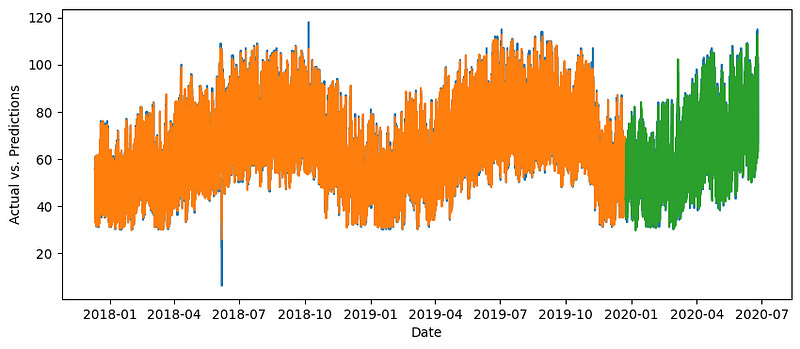
# Plot the actual values in blue
# Plot the forecasts for the training periods in orange
# Plot the forecasts for the test periods in green
plt.figure(figsize=(10,4))
plt.plot(actual_pred['date'], actual_pred[["y",'y_pred_train','y_pred_test']])
plt.xlabel("Date")
plt.ylabel("Actual vs. Predictions")
plt.show()

The orange line is the forecasts for the training periods, and the green line is for the test periods. The two lines appear fitting the actual values well.

Witnessing the predictions, now we want to understand the model itself.

Providing Model explainability

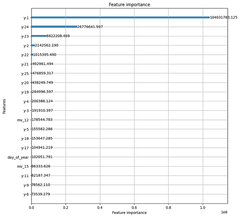
One of the advantages of a tree-based model is its visibility. We can visualize the impacts of the features for forecasts by using a variable importance plot.

lgb.plot_importance(model, max_num_features=20, figsize=(10, 10), importance_type="gain")
plt.show()

The feature importance plot shows the top three influential variables are y_1, y_24, and y_23. The presence of y-1 is expected because electricity consumption typically follows an AR(1) pattern and does not change abruptly. The 12-hour moving average mv_12 appears but is insignificant.

Conclusions

In this chapter, we’ve learned how to create features from a univariate time series. We learned how to frame a univariate time series into a tree-based supervised learning framework. We build a lightGBM model and generate one-step forecasts. We have also demonstrated the use of variable significant plot to increase model explainability.

In next post, we will learn different modeling strategies in producing multi-step-ahead forecasts.

References

Tim Januschowski, Yuyang Wang, Kari Torkkola, Timo Erkkilä, Hilaf Hasson, & Jan Gasthaus (2022). Forecasting with trees. International Journal of Forecasting, 38(4), 1473–1481.
Ke, G., Meng, Q., Finley, T., Wang, T., Chen, W., Ma, W., et al. (2017). LightGBM: A Highly Efficient Gradient Boosting Decision Tree. In I. Guyon, U. V. Luxburg, S. Bengio, H. Wallach, R. Fergus, S. Vish- wanathan, R. Garnett (Eds.), Vol. 30, Advances in neural information processing systems. Curran Associates, Inc..
Time series hourly electricity consumption, Time Series Hourly Electricity consumption(LSTM) | Kaggle
International Institute of Forecasters, https://forecasters.org/resources/time-series-data/
Chris Kuo, My Lecture Notes on Random Forest, Gradient Boosting, Regularization, and H2O.ai, My Lecture Notes on Random Forest, Gradient Boosting, Regularization, and H2O.ai | by Chris Kuo/Dr. Dataman | Analytics Vidhya | Medium