
OpenCV — Histogram Equalization
HOW TO Equalize Histograms Of Images — #PyVisionSeries — Episode #04
INDEX
01 step — Equalizing Manually
02 step — And by using the OpenCV function
What is an Image Histogram?
It is a graphical representation of the intensity distribution of an image. It quantifies the number of pixels for each intensity value considered.
01 step — Equalizing Manually
%matplotlib inlinefrom IPython.display import display, Math, Lateximport numpy as npimport matplotlib.pyplot as pltfrom PIL import Imageimg = Image.open('DATA/einstein.jpg')
plt.imshow(img)<matplotlib.image.AxesImage at 0x1d0b37d2250>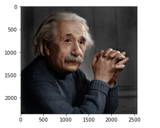
Convert image into a numpy array, so OpenCV can work with:
img = np.asanyarray(img)img.shape(2354, 2560, 3)Converting RGB to Gray Scale:
import cv2img = cv2.cvtColor(img, cv2.COLOR_BGR2GRAY)img.shape(2354, 2560)display the image:
plt.imshow(img, cmap='gray')<matplotlib.image.AxesImage at 0x1d0b415e100>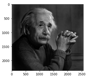
img.max()255
img.min()0
img.shape(2354, 2560)Flatting it out:
flat = img.flatten()# 1 row 2354 x 2560 = 6.026.240flat.shape(6026240,)show the histogram
plt.hist(flat, bins=50)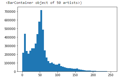
What is Histogram Equalization?
To make it clearer, from the image above, you can see that the pixels seem clustered around the middle of the available range of intensities. What Histogram Equalization does is to stretch out this range.
# formula for creating the histogramdisplay(Math(r'P_x(j) = \sum_{i=0}^{j} P_x(i)'))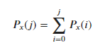
# create our own histogram functiondef get_histogram(image, bins): # array with size of bins, set to zeros histogram = np.zeros(bins) # loop through pixels and sum up counts of pixels for pixel in image: histogram[pixel] += 1 # return our final result return histogramhist = get_histogram(flat, 256)plt.plot(hist)[<matplotlib.lines.Line2D at 0x1d0b4e4da90>]
# create our cumulative sum functiondef cumsum(a): a = iter(a) b = [next(a)] for i in a: b.append(b[-1] + i)
return np.array(b)# execute the fncs = cumsum(hist)# display the resultplt.plot(cs)[<matplotlib.lines.Line2D at 0x1d0b4eafb20>]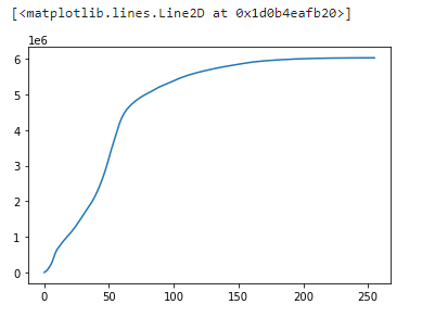
# formula to calculate cumulation sumdisplay(Math(r's_k = \sum_{j=0}^{k} {\frac{n_j}{N}}'))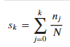
# re-normalize cumsum values to be between 0-255# numerator & denomenatornj = (cs - cs.min()) * 255N = cs.max() - cs.min()# re-normalize the cdfcs = nj / Nplt.plot(cs)[<matplotlib.lines.Line2D at 0x1d0b4f0b7c0>]Casting:
# cast it back to uint8 since we can't use floating point values in imagescs = cs.astype('uint8')plt.plot(cs)[<matplotlib.lines.Line2D at 0x1d0b5f8bd60>]Get CDF:
# get the value from cumulative sum for every index in flat, and set that as img_newimg_new = cs[flat]# we see a much more evenly distributed histogramplt.hist(img_new, bins=50)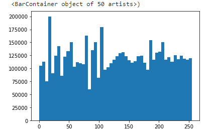
How does it work?
Equalization implies mapping one distribution (the given histogram) to another distribution (a wider and more uniform distribution of intensity values) so the intensity values are spread over the whole range.
# get the value from cumulative sum for every index in flat, and set that as img_newimg_new = cs[flat]# we see a much more evenly distributed histogramplt.hist(img_new, bins=50)
# put array back into original shape since we flattened itimg_new = np.reshape(img_new, img.shape)img_newarray([[233, 231, 228, ..., 216, 216, 215],
[233, 230, 228, ..., 215, 215, 214],
[233, 231, 229, ..., 213, 213, 212],
...,
[115, 107, 96, ..., 180, 187, 194],
[111, 103, 93, ..., 187, 189, 192],
[111, 103, 93, ..., 187, 189, 192]], dtype=uint8)Check it out:
# set up side-by-side image displayfig = plt.figure()fig.set_figheight(15)fig.set_figwidth(15)fig.add_subplot(1,2,1)plt.imshow(img, cmap='gray')# display the new imagefig.add_subplot(1,2,2)plt.imshow(img_new, cmap='gray')plt.show(block=True)Using OpenCV equalizeHist(img) Method
02 step — And by using the OpenCV function
# Reading image via OpenCV and Equalize it right away!img = cv2.imread('DATA/einstein.jpg',0)equ = cv2.equalizeHist(img)Ready! that’s all you need to do!
fig = plt.figure()fig.set_figheight(15)fig.set_figwidth(15)fig.add_subplot(1,2,1)plt.imshow(img, cmap='gray')# display the Equalized (equ) imagefig.add_subplot(1,2,2)plt.imshow(equ, cmap='gray')plt.show(block=True)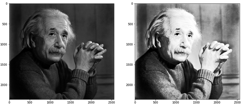
print("That´s it! Thank you once again!\nI hope will be helpful.")That´s it! Thank you once again! I hope will be helpful.
👉Jupiter notebook link :)
👉Github (EX_04)
Credits & References:
Jose Portilla — Python for Computer Vision with OpenCV and Deep Learning — Learn the latest techniques in computer vision with Python, OpenCV, and Deep Learning!
https://www.tutorialspoint.com/dip/histogram_equalization.htm
https://readmedium.com/a-tutorial-to-histogram-equalization-497600f270e2
https://docs.opencv.org/3.4/d4/d1b/tutorial_histogram_equalization.html
https://docs.opencv.org/4.x/d4/d86/group__imgproc__filter.html
https://stackoverflow.com/questions/32838802/numpy-with-python-convert-3d-array-to-2d
https://techtutorialsx.com/2018/06/02/python-opencv-converting-an-image-to-gray-scale/
https://docs.opencv.org/3.4/d4/d1b/tutorial_histogram_equalization.html
https://docs.opencv.org/4.x/d5/daf/tutorial_py_histogram_equalization.html
https://ai.stanford.edu/~syyeung/cvweb/tutorial1.html
https://readmedium.com/histogram-equalization-in-python-from-scratch-ebb9c8aa3f23
Posts Related:
00 Episode#Hi Python Computer Vision — PIL! — An Intro To Python Imaging Library #PyVisionSeries
01 Episode# Jupyter-lab — Python — OpenCV — Image Processing Exercises #PyVisionSeries
02 Episode# OpenCV — Image Basics — Create Image From Scratch #PyVisionSeries
03 Episode# OpenCV — Morphological Operations — How To Erode, Dilate, Edge Detect w/ Gradient #PyVisionSeries
04 Episode# OpenCV — Histogram Equalization — HOW TO Equalize Histograms Of Images — #PyVisionSeries
05 Episode# OpenCV — OpenCV — Resize an Image — How To Resize Without Distortion
07 Episode# YOLO — Object Detection — The state of the art in object detection Framework!
08 Episode# OpenCV — HaashCascate — Object Detection — Viola–Jones object detection framework — #PyVisionSeries