
A Tutorial to Histogram Equalization
Improve your Neural Network’s Performance by Enhancing your Image Data
Image processing is one of the rapidly growing technologies of our time and it has become an integral part of the engineering and computer science disciplines. Among its many subsets, techniques such as median filter, contrast stretching, histogram equalization, negative image transformation, and power-law transformation are considered to be the most prominent. In this tutorial, we will focus on the histogram equalization.
What is a Histogram of An Image?
A histogram of an image is the graphical interpretation of the image’s pixel intensity values. It can be interpreted as the data structure that stores the frequencies of all the pixel intensity levels in the image.
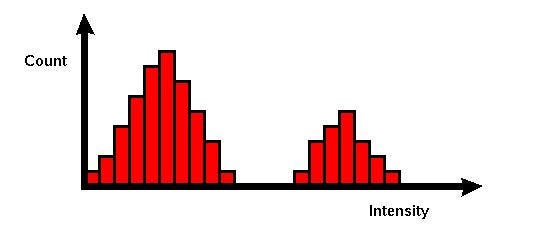
As we can see in the image above, the X-axis represents the pixel intensity levels of the image. The intensity level usually ranges from 0 to 255. For a gray-scale image, there is only one histogram, whereas an RGB colored image will have three 2-D histograms — one for each color. The Y-axis of the histogram indicates the frequency or the number of pixels that have specific intensity values.
What is Histogram Equalization?
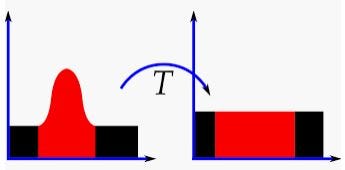
Histogram Equalization is an image processing technique that adjusts the contrast of an image by using its histogram. To enhance the image’s contrast, it spreads out the most frequent pixel intensity values or stretches out the intensity range of the image. By accomplishing this, histogram equalization allows the image’s areas with lower contrast to gain a higher contrast.
Why Do You Use Histogram Equalization?
Histogram Equalization can be used when you have images that look washed out because they do not have sufficient contrast. In such photographs, the light and dark areas blend together creating a flatter image that lacks highlights and shadows. Let’s take a look at an example -
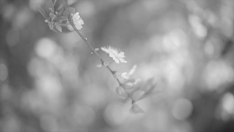
In terms of Photography, this image is, without a doubt, a beautiful bokeh shot of a flower. However, for computer vision and image processing tasks, this photograph doesn’t provide much information since most of its areas are blurry due to lack of contrast.
But not to be worried. We can use histogram equalization to overcome this problem. Let’s take a look!
How to Use Histogram Equalization
Before we get started, we need to import the OpenCV-Python package, a Python library that is designed to solve computer vision problems. In addition to OpenCV-Python, we will also import NumPy and Matplotlib to demonstrate the histogram equalization.
import cv2 as cv
import numpy as np
from matplotlib import pyplot as plt
Next, we will assign a variable to the location of an image and utilize .imread() method to read the image.
path = "...\flower.jpg"img = cv.imread(path)Then, we will use .imshow() method to view the image. Since I am using Jupyter Notebook, I will also add .waitKey(0) and .destroyAllWindows() methods to prevent my notebook from crashing while displaying the image. The image will appear in a separate window of your browser.
cv.imshow('image',img)
cv.waitKey(0)
cv.destroyAllWindows()
Now that our test image has been read, we can use the following code to view its histogram.
hist,bins = np.histogram(img.flatten(),256,[0,256])
cdf = hist.cumsum()
cdf_normalized = cdf * float(hist.max()) / cdf.max()
plt.plot(cdf_normalized, color = 'b')
plt.hist(img.flatten(),256,[0,256], color = 'r')
plt.xlim([0,256])
plt.legend(('cdf','histogram'), loc = 'upper left')
plt.show()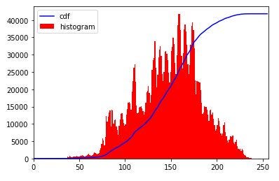
As displayed in the histogram above, the majority of the pixel intensity ranges between 125 and 175, peaking around at 150. However, you can also see that the far left and right areas do not have any pixel intensity values. This reveals that our test image has poor contrast.
To fix this, we will utilize OpenCV-Python’s .equalizeHist() method to spreads out the pixel intensity values. We will assign the resulting image as the variable ‘equ’.
equ = cv.equalizeHist(img)Now, let’s view this image.
cv.imshow('equ.png',equ)
cv.waitKey(0)
cv.destroyAllWindows()
If you compare the two images above, you will find that the histogram equalized image has better contrast. It has areas that are darker as well as brighter than the original image.
Now, let’s compare the original and the equalized histograms. We will use the same code that we used to view the original histogram.
hist,bins = np.histogram(equ.flatten(),256,[0,256])
cdf = hist.cumsum()
cdf_normalized = cdf * float(hist.max()) / cdf.max()
plt.plot(cdf_normalized, color = 'b')
plt.hist(equ.flatten(),256,[0,256], color = 'r')
plt.xlim([0,256])
plt.legend(('cdf','histogram'), loc = 'upper left')
plt.show()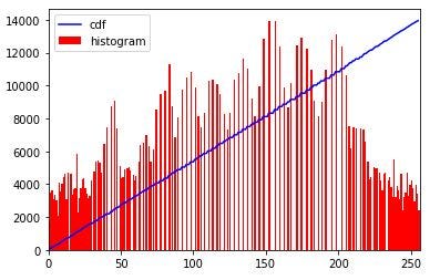
Unlike the original histogram, the pixel intensity values now range from 0 to 255 on the X-axis. In a way, the original histogram has been stretched to the far ends. You may also notice that the cumulative distribution function (CDF) line is now linear as opposed to the original curved line.
In addition to the ordinary histogram equalization, there are two advanced histogram equalization techniques called -
- Adaptive Histogram Equalization
- Contrastive Limited Adaptive Equalization
Adaptive Histogram Equalization (AHE)
Unlike ordinary histogram equalization, adaptive histogram equalization utilizes the adaptive method to compute several histograms, each corresponding to a distinct section of the image. Using these histograms, this technique spread the pixel intensity values of the image to improve the contrast. Thus, adaptive histogram equalization is better than the ordinary histogram equalization if you want to improve the local contrast and enhance the edges in specific regions of the image.
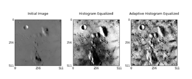
One limitation of AHE is that it tends to overamplify the contrast in the near-contrast regions of the image.
Contrastive Limited Adaptive Equalization
Contrastive limited adaptive equalization (CLAHE) can be used instead of adaptive histogram equalization (AHE) to overcome its contrast overamplification problem. In CLAHE, the contrast implication is limited by clipping the histogram at a predefined value before computing the CDF. This clip limit depends on the normalization of the histogram or the size of the neighborhood region. The value between 3 and 4 is commonly used as the clip limit.
Conclusion
Histogram equalization is a valuable image preprocessing technique that can be used to obtain extra data from images with poor contrast. With this technique, I hope you can improve the performances of your computer vision and machine learning tasks.


