Summary

The web content provides a step-by-step guide to setting up a Python environment for image processing using OpenCV and Jupyter Notebooks, and demonstrates basic image manipulation techniques using Python libraries such as PIL, Numpy, and Matplotlib.

Abstract

The website outlines a comprehensive tutorial for individuals interested in computer vision with Python. It begins by instructing users on how to create a conda environment and set up Jupyter Notebooks for running OpenCV code. The guide includes downloading necessary files and creating a dedicated directory for the project. It then proceeds to demonstrate how to create a virtual environment using a provided .yml file, which ensures all required libraries are installed. The tutorial transitions into practical exercises, showcasing how to manipulate images using the Pillow library, convert images to Numpy arrays, and visualize different color channels with Matplotlib. The content emphasizes hands-on learning by guiding users through the process of isolating and displaying individual color channels (red, green, and blue) from an image, and explains how these channels contribute to the overall color composition of the image. The article concludes with a teaser for the next episode on OpenCV basics and provides links to the Jupyter notebook and GitHub repository for further exploration.

Opinions

The author believes in the importance of a structured setup for Python environments to ensure reproducibility and ease of use when working with computer vision projects.
There is an emphasis on the practical application of theoretical knowledge, encouraging users to engage with the code and visualize results as they learn.
The tutorial is designed to be beginner-friendly, providing clear instructions and visual aids to facilitate understanding.
The author suggests that understanding how to manipulate and analyze image data at the pixel level is fundamental to computer vision tasks.
By highlighting the use of Jupyter Notebooks, the author conveys the value of an interactive coding environment for experimentation and learning.
The tutorial promotes the idea that breaking down an image into its constituent color channels can provide insights into the image's composition and color information.
The mention of upcoming episodes on OpenCV basics and more advanced topics like object detection indicates the author's commitment to providing a series of educational resources for those interested in deepening their knowledge in computer vision.

OpenC V— Jupyter-lab — Python

Image Processing Exercises — #PyVisionSeries — Episode #01

Let´s create a conda environment for running python OpenCV code.

We are working with Jupyter Notebook :)

Please, first, download Anaconda package for Data Science.

Download all the files for this project.

Now folow theses steps:

00step — Create Directory to work with

Create anywhere on your windows computer a directory (python_opencv)

Now type on prompt:

cd Downloads
mkdir python_opencv

cd python_opencv
cd

and paste these file inside:

python_opencv.yml

DATA [Directory containing the images]

Yml file will import all the libs that you will need for OpenCV via Conda.

01step — Create a Virtual Environment

In your prompt (inside python_opencv dir):

conda env create -f python_opencv.yml

02 step— Run Jupyter Notebook:

jupyter-lab

If all goes well, you will find this screen open in your browse:

keep prompt screen open. Now you are ready to go!

Before we dive into OpenCV, Let´s see how to manipulate Image w/ Pure Python!

GOTO

File > New > Notebook 
[Python3 ipykernel]

Rename it as 01_cv_00.ipynb,

and Type:

PILLOW LIB

import numpy as np

Importing Numpy as well Matplotlib:

import matplotlib.pyplot as plt

%matplotlib inline

Importing Pillow lib:

from PIL import Image

Save this image DATA to your directory: 00_puppy.jpg (or whatever you like:)

pic = Image.open('DATA/00_puppy.jpg')

Type:

pic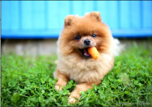

type(pic)

PIL.JpegImagePlugin.JpegImageFile

To work with Numpy we must convert JPEG image into Numpy Array. Here is how to:

pic_arr = np.asanyarray(pic)

This now is a Numpy Array:

type(pic_arr)

numpy.ndarray

It’s Shaped as:

pic_arr.shape

(551, 789, 3)

Use MatPlotLib to show the image:

plt.imshow(pic_arr)
<matplotlib.image.AxesImage at 0x23b0bf38eb0>

It’s Shaped as:

pic_arr.shape
(551, 789, 3)

Note that there’s three channels here, the red, the green and the blue.

Each one has its array, (551, 789) for Red , (551, 789) for Green and, (551, 789) for Blue. 3-D arrays.

Let’s actually access one of these channels by itself:

For RED:

pic_red = pic_arr[:,:,0]

Showing the img:

# RED CHANNEL VALUES 0-255 0 = NO COLOR ALUE 255 = FULL COLOR

plt.imshow(pic_red, cmap='gray')

<matplotlib.image.AxesImage at 0x23b0beb99a0>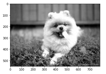

Notice that the dog’s coat is reddish, so it appears white in the image

So that means when we’re actually viewing this in grayscale, the closer to white that means more red for this particular image.

For GREEN:

pic_green = pic_arr[:,:,1]

plt.imshow(pic_green, cmap='gray')

<matplotlib.image.AxesImage at 0x23b0d18a2b0>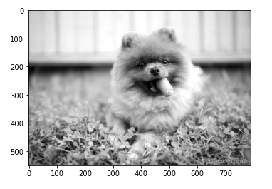

Notice that the grass is green, so it appears white in the image, at the ends

For BLUE:

pic_blue = pic_arr[:,:,2]

plt.imshow(pic_blue, cmap='gray')

<matplotlib.image.AxesImage at 0x23b0d1d8490>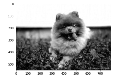

Note that the container behind is blue, so it appears very clear in the image

So, here we’re displaying the three different channels as grayscale.

Now let´s zeroed GB and stick with R channel

pic_copy = pic_arr.copy()

Zeroed out the Green Channel:

pic_copy[:,:,1] = 0

Zeroed out the Blue Channel:

pic_copy[:,:,2] = 0

Shows up the RED channel:

plt.imshow(pic_copy)

Here the other channels were zeroed, and red prevails

We went ahead and zeroed out the Green Channel as well as the Blue Channel, which is why this picture only shows up with the red.

pic_copy.shape

(1044, 1000, 3)

There are 3 channel, yet! because we’re seeing all three channels at once instead of just one channel.

What we did was zeroed two channels, but the arrays remain intact even if their values have been set to zero

print("That's it! Thanks for reading. Next Episode: OpenCV  Basics\nSee you soon!")

That's it! Thanks for reading. Next Episode: OpenCV  Basics
See you soon!

👉Jupiter notebook link :)

👉Github (EX_01)

Credits & References:

Jose Portilla — Python for Computer Vision with OpenCV and Deep Learning — Learn the latest techniques in computer vision with Python, OpenCV, and Deep Learning!

Posts Related:

00 Episode#Hi Python Computer Vision — PIL! — An Intro To Python Imaging Library #PyVisionSeries

01 Episode# Jupyter-lab — Python — OpenCV — Image Processing Exercises #PyVisionSeries

02 Episode# OpenCV — Image Basics — Create Image From Scratch #PyVisionSeries

03 Episode# OpenCV — Morphological Operations — How To Erode, Dilate, Edge Detect w/ Gradient #PyVisionSeries

04 Episode# OpenCV — Histogram Equalization — HOW TO Equalize Histograms Of Images — #PyVisionSeries

05 Episode# OpenCV — OpenCV — Resize an Image — How To Resize Without Distortion

07 Episode# YOLO — Object Detection — The state of the art in object detection Framework!

08 Episode# OpenCV — HaashCascate — Object Detection — Viola–Jones object detection framework — #PyVisionSeries