Temporal Fusion Transformer for Interpretable Time Series Predictions

We shop at retail businesses like Walmart, Target, and Best Buy. We buy from department stores like Macy’s, Nordstrom, and Sears. We visit supermarkets like Kroger, Safeway, and Whole Foods. We surf online retailers like Amazon and eBay. We expect a product to arrive at our doors on time. We frown if a product is out of stock. These businesses have several aspects in common: they sell hundreds and thousands of products, and they all rely on efficient planning. They all rely on good data science models for planning guidance. These types of data science models need to provide forecasts for thousands of products. The forecasts cannot be just one period but should be multiple periods. The forecasts should have prediction intervals to quantify uncertainty.

This chapter introduces a Transformer-based forecasting model that can deliver forecasts for multiple products, multiple periods, and probabilistic forecasts. It is the Temporal Fusion Transformer (TFT) model. TFT has been shown to outperform other models in certain tasks. Its efficiency, flexibility, and interpretability make it a valuable asset for a wide range of applications. Its title is intriguing too since its introduction in 2019 by Lim, Arik, Loeff, and Pfister [1]. “Temporal” refers to its handling of time-related data or sequential data that have temporal dependencies. “Fusion” captures its design that blends information from multiple data sources or features. And “Transformer” because it is a Transformer-based model. The Transformer model of the seminal paper “Attention is All You Need” (2017) [2] has been the backbone for all the modern large language models (LLMs). You can reference the previous chapter “From RNN/LSTM to Temporal Fusion Transformers and Lag-Llama”.

Today’s data science models are intricate machines, and may still be in their infant stage towards total enigmatic labyrinths. In the meantime, the data science community requires model transparency and interpretability. They ask questions about how the model makes the predictions. Model interpretability is an active research area to ensure responsible model predictions, as I have covered in “An Explanation for eXplainable AI” and in the book “The explainable AI”. Model Interpretability is TFT’s salient feature that provides insights into how it makes predictions. It explains which past-time steps are most influential in predicting future values. Later in the code example we will see the variable importance plots that explain how the model makes predictions.

This chapter will walk you through a real data case to build a TFT model. We will cover the following topics:

• Building global time series models
• The architecture of TFT
• Software requirements
• Data
• Data Conversion to the Darts Python library
• Modeling
• Forecasting
• Plotting
• Model Interpretability

Upon the completion of this chapter, you will be able to apply TFT to your future cases and explain the benefits of of TFT.

Building Global Time Series Models

The thousands of products at Walmart or Amazon mean there are thousands of time series. If all the time series are modeled together, the model is a global model. If each time series is modeled as a univariate time series model, it is a local model. It is worth noting here that, in practice, you may build separate global models for each product category, in which there may be thousands of products.

What’s the advantage of a global model? A global model can capture common patterns and relationships across multiple time series, which can improve the accuracy of forecasts for individual time series. Global models can also be useful when there is a limited amount of data available for a single time series, as they can leverage information from other time series to improve forecasts. For example, a new product does not have history. But it can leverage the features of similar products in the same category.

On the other hand, a local model is trained on a single time series and can capture unique patterns and trends that may not be present in other time series. Local models can be useful when there are significant differences between time series.

The Temporal Fusion Transformer (TFT) model is a global model, meaning that it models the relationships between different time series, rather than modeling each time series independently. The idea behind TFT is that the relationships between time series can be captured by a shared representation that captures the underlying patterns and trends across all series. By modeling the joint distribution of all series, TFT can capture complex patterns and relationships that would be difficult to model with a local model that only considers a single time series.

I need to advise you that the next section on the architecture of TFT is long. Alternatively, you can jump directly to the “Software requirement” section to learn the modeling, then come back to the architecture of TFT.

The Architecture of TFT

Figure (A) shows the architecture of TFT of the original paper [1]. The diagram appears intimidating. We will cover the blocks step by step.

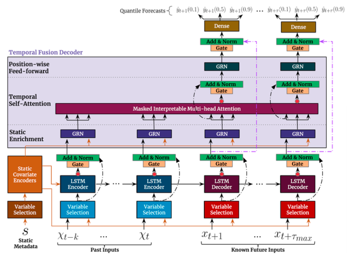
The way to read Figure (A) is from the bottom. You will start with the inputs at the bottom. Then move up one row for the “Variable Selection” boxes. Then move up one row for the “Encoders” boxes, and so on. The final output is the quantile forecasts at the top.

The Input Data

Time series data can be broadly grouped into three types:

1. The first group is the static metadata such as store location or product category that do not change over time.
2. The second group is past inputs of k periods.
3. The third group is other covariates such as holiday flags, day of the week or month, scheduled promotion events. Because we will predict the future 𝛕 periods, these covariates should be prepared or known up to the t+ 𝛕 period.

Variable Selection Network

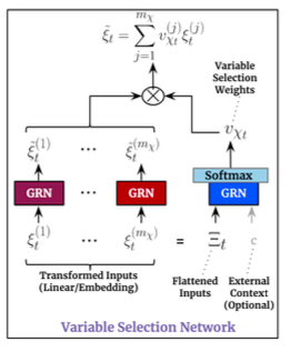
Not all input data are related with the target data. The Variable Selection Networks (VSNs) determine which input data are most relevant for forecasting. It is an intuitive design of TFT. VSNs dynamically select a subset of the most relevant input data at each time step for forecasting. This dynamic feature selection mechanism allows the model improve forecasting accuracy. However, we do not know which of the inputs are relevant to the target in advance, nor do we know the precise relationship whether it is linear or non-linear. How can we identify the relevant inputs? VSNs allow the model to be flexible to select input variables and discard information as needed. Figure (B) shows a Variable Selection Network. There are Gated Residual Networks for each of the input features. The “Variable Selection Weights” in the diagram are the weights for variable importance. The weights are determined during the training process.

Let’s understand Gated Residual Networks (GRNs).

Gated Residual Network (GRN)

The Gated Residual Networks (GRNs) are used throughout TFT to enhance the model’s ability to capture complex temporal patterns and dependencies in time series data. A GRN has the Gated mechanism and Residual Connections as shown in Figure (C). The gating mechanism allows the model to adaptively adjust the importance of different features at each layer. These gating functions typically take the form of sigmoidal activation functions, producing values between 0 and 1. They determine how much of the information from the previous layer should be passed through to the next layer, allowing the model to selectively retain or discard information as needed.

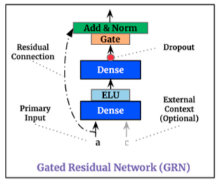
Figure (C) has a dashed line for the residual connection. The output of the previous layer(s) is added to the output of the current layer. This mechanism helps address the vanishing gradient problem. Also, the additions of the outputs of previous and subsequent layers through residual connections, the GRN has mixed the input features and is able to capture the non-linear interactions between features. That’s what the name “Fusion” is coined.

After explaining the row of VSNs in Figure (A), let’s move up one row to the Static Covariate Encoders.

Static Covariate Encoders

The static covariate encoders convert categorical static covariates into numerical representations. This embedding process is similar to word embeddings in natural language processing. Each categorical variable is mapped to a high-dimensional vector in an embedding space. This embedding process captures the semantic relationships between different categories. You are advised to read Chapter 1 to 3 in the book “The Handbook of NLP with Gensim” [3], which gives friendly explanations for text representation and word embedding.

LSTM Encoders

In the previous chapter “From RNN/LSTM to Temporal Fusion Transformers and Lag-Llama” we have explained that we cannot use a Transformer model directly for time series data. This is merely because time series data and language data are different. How to encode time series data? We know time series data have unique temporal dependencies and patterns within the time series data. The encoders for time series data are the Long Short-Term Memory (LSTM) networks. LSTM encoders are a type of recurrent neural network (RNN) architecture known for their ability to effectively model sequential data. As the LSTM encoders process the input time series data, they extract relevant features and learn meaningful representations of the temporal dynamics present in the data.

The Arrow of the Static Covariate Encoders to the LSTM Encoders

You probably have noticed the arrow of the static covariate encoders to the LSTM encoders in Figure (A). It means the numerical representations of the static covariates are concatenated with the temporal features in LSTM encoders. This concatenation process combines the information from both the static covariates and the temporal features. This helps the model to leverage both temporal and static information for accurate forecasting. For example, later in the code example one of the static covariates is store. The store sales can vary due to store locations. the combination of the store information with past temporal features makes the model flexible to predict store-specific sales accurately.

LSTM Decoders

The covariates for the future 𝛕 periods are fed into the LSTM decoders. Similar to LSTM encoders, LSTM decoders are capable of capturing temporal dependencies and patterns within the data.

Static Enrichment with GRNs

Now let’s move up to the static enrichment in Figure (A). There is a set of GRNs to take the inputs from the LSTM encoders, and another set of GRNs to take the inputs from the LSTM decoders. Both sets of GRNs also take the static covariates in vector forms as inputs too. Again, the static enrichment of GRNs enables the TFT to make more accurate forecasts by leveraging both temporal dependencies and static covariate information.

Temporal Multi-head Self-Attention

The temporal self-attention mechanism lets the model to attend to different time steps in the same input sequence and learn complex relationships between them. The temporal self-attention mechanism operates similarly to the standard self-attention mechanism used in transformer architectures. At each time step in the input sequence, the temporal self-attention mechanism computes attention weights that determine how much focus to place on each time step when encoding the input sequence. Time steps that are more relevant or informative for the forecasting task receive higher attention weights, while less relevant time steps receive lower attention weights. These weights are the ingredients for TFT to perform model interpretability. Later in the code example you will see how we visualize the self-attention weights.

Notice self-attention mechanism is multi-head. It allows the model to attend to different aspects of the input sequence simultaneously. A single self-attention means paying attention to some parts within the same time series segment. Similarly, instead of computing attention only once, the multi-head lets the model to compute attention multiple times in parallel. Each attention head learns a distinct set of attention weights to capture different types of relationships within the input sequence. By using multiple attention heads, the model can capture diverse patterns and dependencies more effectively.

Position-wise Feed-forward Network

Unlike traditional feed-forward networks, which process the entire input sequence simultaneously, the position-wise FFN in the TFT processes each position in the input sequence independently. This position-wise processing allows the model to capture position-specific information and interactions within the input sequence. The feed-forward network applies non-linear activation functions (such as ReLU or GELU).

Add & Norm

There are a few “Add & Norm” blocks. The “Add & Norm” technique enhances the training stability and convergence speed of the TFT model. The purpose of the “Add” operation is to allow the model to retain the original information from the input while also incorporating the transformed information from the output. By adding the input to the output of the layer, the model can ensure that the original information is preserved throughout the transformation process. This helps mitigate the vanishing gradient problem.

Quantile Regression Outputs for Multiple Periods

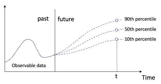
Finally, the model generates quantile forecasts for multiple future time steps simultaneously. The quantile regression estimates multiple quantiles (e.g., 10th, 50th, and 90th percentiles) to quantify different levels of uncertainty, as illustrated in Figure (D). This part is the same as the quantile regression techniques in the previous chapters “Linear Regression for Multi-period Probabilistic Forecasting” and “Tree-based XGB, LightGBM, and CatBoost Models for Multi-period Time Series Probabilistic Forecasting”.

Optimization

The optimization algorithm of TFT is the standard neural network algorithm. It uses stochastic gradient descent (SGD) or its variants. It defines the loss function between actual and predicted values. Backpropagation is then used to compute the gradients of the loss with respect to the model parameters. The gradients are used to update the parameters through gradient descent, where the learning rate determines the step size. Mini-batch training is employed to speed up training and improve generalization. Regularization techniques, such as L1 or L2 regularization, can be applied to prevent overfitting. Learning rate scheduling adjusts the learning rate over time. The optimization algorithm iteratively performs these steps until a stopping criterion, such as a maximum number of epochs or desired performance level, is met.

Let’s now use a real data case to build a TFT model. The Python notebook is available via this Github link for download.

Software requirements

You will need to install the Darts Python library. This book dedicates a chapter “Time Series Data Formats Made Easy” to orient you with the Darts data format. This book also demonstrates Darts in the following chapters of this book:

• Time Series Data Formats Made Easy
• Linear Regression for Multi-period Probabilistic Forecasting
• Tree-based XGB, LightGBM, and CatBoost Models for Multi-period Time Series Probabilistic Forecasting
• Application: Amazon’s DeepAR for Stock Forecasts

Let’s import the necessary libraries.

import pandas as pd
import numpy as np
from datetime import timedelta
import matplotlib.pyplot as plt

from darts import TimeSeries
from darts.dataprocessing.pipeline import Pipeline
from darts.models import TFTModel
from darts.dataprocessing.transformers import Scaler
from darts.utils.timeseries_generation import datetime_attribute_timeseries
from darts.utils.likelihood_models import QuantileRegression
from darts.dataprocessing.transformers import StaticCovariatesTransformer, MissingValuesFiller

Data Preparation

We will use the store sales at Favorita stores in Ecuador. The dataset is available on Kaggle. The dataset has thousands of product families sold at the chain stores. The training data includes dates, store and product information, whether that item was being promoted, as well as the sales numbers. Additional files include supplementary information that may be useful in building your models.

The preceding code merges multiple files.

# Read csv
path = 'data/store-sales-time-series-forecasting'
data = pd.read_csv(path + '/train.csv', delimiter=",")
holidays= pd.read_csv(path + '/holidays_events.csv', delimiter=",").drop('type', axis=1)
stores= pd.read_csv(path + '/stores.csv', delimiter=",")
transactions= pd.read_csv(path + '/transactions.csv', delimiter=",")
# Merge files
holidays['holiday_flag']=1
data = data.merge(holidays, on='date', how='left')
data= data.merge(stores, on='store_nbr', how='left')
data = data[data['date']!='2013-01-01'] # Bad data
data= data.merge(transactions, on=['date', 'store_nbr'], how='left')
# Basic data manipulation
data['date'] = pd.to_datetime(data["date"])
data = data.drop_duplicates(subset=['date','store_nbr', 'family'], keep='last') 
data.loc[data['holiday_flag'].isna(),'holiday_flag']=0
data['year'] = data['date'].dt.year 
data.columns

The data have these columns:

• store_nbr: the store number
• family: The product family
• sales: the total sales for a product family at a store and a date
• onpromotion: the total number of items in a product family that were being promoted at a store and a date
• holiday_flag: flags for the holidays

There are hundreds of time series in the data because each product in a store is a time series. For illustration purposes, we will select the four largest stores and four largest product families to build the global model. The preceding code selects the 16 time series data and then splits them into training and test data.

data.groupby('store_nbr')['sales'].agg(['count','sum']).sort_values(by='sum',ascending=False).head()
# Store_nbr: 44, 45, 47, 3 are large stores. We will just do the forecasting for them.

data.groupby('family')['sales'].agg(['count','sum']).sort_values(by='sum',ascending=False).head()
# Product family: 'GROCERY I','BEVERAGES','PRODUCE','CLEANING' are large categories. We will just do the forecasting for them.

data = data[ ( data['store_nbr'].isin([44, 45, 47, 3]) ) & 
             ( data['family'].isin(['GROCERY I','BEVERAGES','PRODUCE','CLEANING']) ) &
             ( data['date'].dt.year >=2016)
           ]

# Split data into train and test
train = data[data['date']<pd.to_datetime('2017-07-15')]
test = data[data['date']>=pd.to_datetime('2017-07-15')]
[train['date'].nunique(),test['date'].nunique()] # [560, 32]

Data Conversion to Darts

To build a global model for multiple time series, we need to structure the data that contain multiple time series. This is engineered conveniently by Darts, as explained in the chapter “Time Series Data Formats Made Easy”. The most granular level of the time series is at the store and product family level, so we specify the grouping as “store_nbr” and “family”. These two variables are not just grouping variables, they can serve as predictors as well. For example, a certain store or product family may sell more than other stores or product families. The two variables can capture the store- and product-specific information.

TIME_COL = "date"
TARGET = "sales"
STATIC_COLS = ['store_nbr', 'family'] 
FREQ = "D"
FORECAST_HORIZON = test['date'].nunique() 
COVARIATES = ['onpromotion','holiday_flag']
SCALER = Scaler()
TRANSFORMER = StaticCovariatesTransformer()
PIPELINE = Pipeline([SCALER, TRANSFORMER])

The target is “sales”, and the covariates are “onpromotion” and “holiday_flag”. The .from_group_dataframe() function in Darts is a convenient tool that can fill in missing values or extrapolate values.

# read train and test datasets and transform train dataset
train_darts = TimeSeries.from_group_dataframe(df=train, 
                                              group_cols=STATIC_COLS, 
                                              time_col=TIME_COL, 
                                              value_cols=TARGET, 
                                              freq=FREQ, 
                                              fill_missing_dates=True, 
                                              fillna_value=0)
test_darts = TimeSeries.from_group_dataframe(df=test, 
                                             group_cols=GROUP_COLS, 
                                             time_col=TIME_COL, 
                                             value_cols=TARGET, 
                                             freq=FREQ, 
                                             fill_missing_dates=True, 
                                             fillna_value=0)

[len(train_darts[0]), len(test_darts[0])] # [561, 32] is the number of periods for the training and test data

A time index contains a lot of hidden information. Certain events may happen on certain days. For example, customers usually shop more on weekends, and summer months usually show more demand for outdoor products. We can use the time index to create more covariates. The preceding code generates indicators for the 12 months and 52 weeks in a year.

create_covariates = []
for ts in train_darts:
    # Add the month and week as a covariate
    covariate = datetime_attribute_timeseries(
        ts,
        attribute="month",
        one_hot=True,
        cyclic=False,
        add_length=FORECAST_HORIZON,
    )
    covariate = covariate.stack(
        datetime_attribute_timeseries(
            ts,
            attribute="week",
            one_hot=True,
            cyclic=False,
            add_length=FORECAST_HORIZON,
        )
    )
    store = ts.static_covariates['store_nbr'].item()
    family = ts.static_covariates['family'].item()
    # create covariates
    other_cov = TimeSeries.from_dataframe(data[(data['store_nbr'] == store) & (data['family'] == family)], time_col=TIME_COL, value_cols=COVARIATES, freq=FREQ, fill_missing_dates=True)
    covariate = covariate.stack(MissingValuesFiller().transform(other_cov))

    create_covariates.append(covariate)

create_covariates[0].columns

#Index(['month_0', 'month_1', 'month_2', 'month_3', 'month_4', 'month_5',
#       'month_6', 'month_7', 'month_8', 'month_9', 'month_10', 'month_11',
#       'week_0', 'week_1', 'week_2', 'week_3', 'week_4', 'week_5', 'week_6',
#       'week_7', 'week_8', 'week_9', 'week_10', 'week_11', 'week_12',
#       'week_13', 'week_14', 'week_15', 'week_16', 'week_17', 'week_18',
#       'week_19', 'week_20', 'week_21', 'week_22', 'week_23', 'week_24',
#       'week_25', 'week_26', 'week_27', 'week_28', 'week_29', 'week_30',
#       'week_31', 'week_32', 'week_33', 'week_34', 'week_35', 'week_36',
#       'week_37', 'week_38', 'week_39', 'week_40', 'week_41', 'week_42',
#       'week_43', 'week_44', 'week_45', 'week_46', 'week_47', 'week_48',
#       'week_49', 'week_50', 'week_51', 'onpromotion', 'holiday_flag'],
#      dtype='object', name='component')

How do they look like? We still can convert the Darts data back to a Pandas data frame to take a look. They are simple binary indicators.

TimeSeries.pd_dataframe(create_covariates[0]).tail()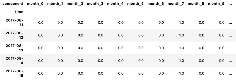

Likewise, we can convert the target data “sales” back to a Pandas data frame to take a look:

TimeSeries.pd_dataframe(train_darts[15]).tail()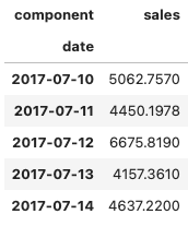

We want to standardize the data before modeling. This practice is common in many data science models. The preceding code builds a scaler according to the training data. This scaler will be applied to the test data later. A novice learner may commit the mistake that scaling the training and test data independently. If you would like to avoid such errors, you can reference the post “Avoid These Deadly Modeling Mistakes that May Cost You a Career”.

# scale data and transform static covariates
# Notice SCALER is before PIPELINE because PIPELINE includes SCALER
train_transformed = PIPELINE.fit_transform(train_darts)
# scale covariates
covariates_transformed = SCALER.fit_transform(create_covariates)

Now let’s build the model.

Modeling

The declaration of the model follows contains the standard neural-network hyperparameters, as well as time-series specific hyperparameters. To increase readability, I group the hyperparameters into:

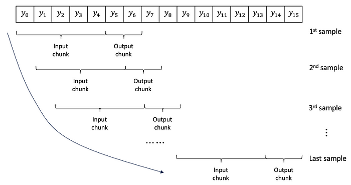
• Hyper-parameters for data preparation: This group refers to input_chunk_length and output_chunk_length in the code. They are about the generation of samples from univariate series. For illustration purposes, Figure (E) shows samples created from the series y0 to y15. Each sample contains an input chunk and an output chunk. Assume the input chunk length is 5 and the output chunk length is 2. The first sample has y0 — y4 as the input chunk and y5, y6 as the output chunk. The window slides alone the series to create samples until the end of the series.

• Hyper-parameters for time series: We will use quantile regression to produce the prediction intervals. This is an important feature for the model to produce prediction uncertainty.
• Hyper-parameters for model architecture: You can fine-tune a range of values for the model specifications including the number of hidden layers, the number of attention of heads, and the number of LSTM layers.
• Hyper-parameters for optimization: This is the standard neural-network hyperparameters. I add the explanations for these hyperparameters in the Appendix.

TFT_params = {
    # hyperparameters for data preparation 
    "input_chunk_length": 52, # number of weeks to lookback
    "output_chunk_length": FORECAST_HORIZON,

    # time series hyperparameters 
    "likelihood": QuantileRegression(quantiles=[0.25, 0.5, 0.75]),
    
    # Hyperparameters for model architecture
    "use_static_covariates": True,
    "hidden_size": 2,
    "lstm_layers": 2,
    "num_attention_heads": 1,

    # Hyperparameters for optimization
    "dropout": 0.1,
    "batch_size": 16,
    "n_epochs": 3,
    "random_state": 42,
    "optimizer_kwargs": {"lr": 1e-3},
}

tft_model = TFTModel(**TFT_params)
tft_model.fit(train_transformed, # The training periods
              future_covariates=covariates_transformed, # The entire periods
              verbose=False)

Once the model is trained, we will use it to forecast.

Forecasting

The forecasting step is straightforward. One thing to remember is the “future_covariates”. The covariates already have the future covariates including Month 1–12, Week 1–52, and holiday flags. It also includes other known covariates like the “onpromotion” flag that will be imported externally.

The predicted values are scaled values. Remember to inverse the scaled values back to the original scale.

# Get the prediction that is scaled
scaled_pred = tft_model.predict(n=FORECAST_HORIZON, 
                                series=train_transformed, # The training periods
                                num_samples=50, 
                                future_covariates=covariates_transformed # The entire periods
                               )

# Transform the scaled prediction to the normal scale
prediction = PIPELINE.inverse_transform(scaled_pred)

Up to now, we have completed the global model for our case and provided the forecasts with uncertainty.

Plotting

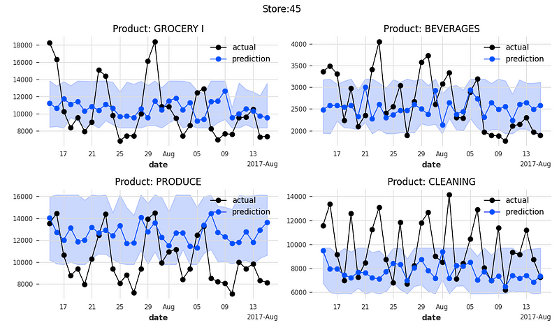
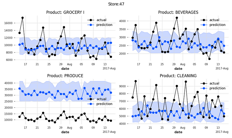
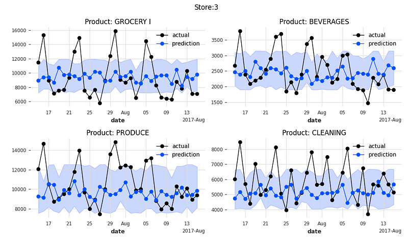
Let’s plot the actual sales, the predicted sales, and the prediction intervals at the 25% and 75% quantiles. The function below plots the 4 product families of a store.

def plot_it():
    fig, axs = plt.subplots(2, 2, figsize=(10, 6), dpi=100)
    ax0 = axs[0,0]
    ax1 = axs[0,1]
    ax2 = axs[1,0]
    ax3 = axs[1,1]
    
    plt.suptitle("Store:" +  str(store) , fontsize=12)
    
    val0[: pred0.end_time()].plot(ax=ax0, label="actual", marker='o', linewidth=1)
    pred0.plot(ax = ax0, low_quantile=0.25, high_quantile=0.75, label="prediction", marker='o',linewidth=1,alpha=0.2 )
    ax0.title.set_text('Product: '+family[0])
    
    val1[: pred1.end_time()].plot(ax=ax1, label="actual", marker='o', linewidth=1)
    pred1.plot(ax = ax1, low_quantile=0.25, high_quantile=0.75, label="prediction", marker='o',linewidth=1,alpha=0.2 )
    ax1.title.set_text('Product: '+family[1])
    
    val2[: pred2.end_time()].plot(ax=ax2, label="actual", marker='o', linewidth=1)
    pred2.plot(ax = ax2, low_quantile=0.25, high_quantile=0.75, label="prediction", marker='o',linewidth=1,alpha=0.2 )
    ax2.title.set_text('Product: '+family[2])
    
    val3[: pred3.end_time()].plot(ax=ax3, label="actual", marker='o', linewidth=1)
    pred3.plot(ax = ax3, low_quantile=0.25, high_quantile=0.75, label="prediction", marker='o',linewidth=1,alpha=0.2 )
    ax3.title.set_text('Product: '+family[3])
    fig.tight_layout()
    plt.show()


store_nbr = [44, 45, 47, 3]
family = ['GROCERY I', 'BEVERAGES', 'PRODUCE', 'CLEANING']

for i in range(0,16,4):
    k = int(i/4)
    store = store_nbr[k]
    pred0 = prediction[i]
    pred1 = prediction[i+1]
    pred2 = prediction[i+2]
    pred3 = prediction[i+3]
    val0 = test_darts[i]
    val1 = test_darts[i+1]
    val2 = test_darts[i+2]
    val3 = test_darts[i+3]
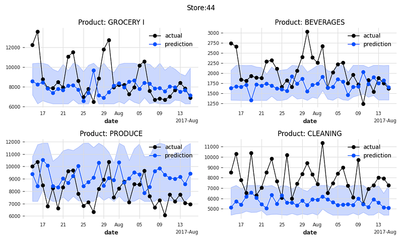
    plot_it()

The following 16 exhibits are the actual values and the predicted values for 4 product categories of 4 stores.

An important feature of TFT is model interpretability. Let’s find out.

Model Interpretability

TFT provides interpretability through the use of self-attention mechanisms. Self-attention mechanisms mean they attend to different parts of the same input sequence when making predictions. By attending to specific features or time steps, the model can highlight their relative importance in the forecasting process. This helps in understanding the underlying factors driving the forecasts and gaining insights into the data. To do this, we will use the TFTExplainer() function.

from darts.explainability import TFTExplainer

explainer = TFTExplainer(
    tft_model,
    background_series=train_transformed[1],
    background_future_covariates=dynamic_covariates_transformed[1],
)
explainability_result = explainer.explain()

Some of you may notice the function name “explainer” resembles the explainer function in SHAP values. Although they function differently, they have the same goal to explain the model itself. The SHAP explainer or other techniques can be found in “An Explanation for eXplainable AI” and the book “The explainable AI”.

We are ready to visualize the attention weights. These visualizations can reveal patterns and relationships between different features or time steps. The first variable importance chart is the encoder importance.

Encoder variable importance measures of how much each input variable contributes to the accuracy of the forecasts. It is calculated using the attention mechanism, which allows the model to focus on the most relevant input variables at each time step.

plt.rcParams["figure.figsize"] = (10,5)
plt.barh(data=explainer._encoder_importance.melt().sort_values(by='value').tail(10), y='variable', width='value')
plt.xlabel('Importance')
plt.ylabel('Feature')
plt.title('Encoder Importance')
plt.show()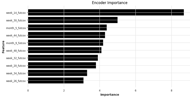

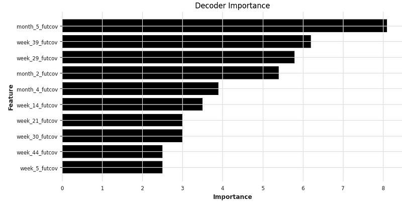
In the TFT model, the decoder consists of multiple layers, each of which consists of a self-attention mechanism followed by a feed-forward neural network (FFNN). The self-attention mechanism allows the model to attend to different parts of the input sequence and weigh their importance when generating the output sequence. The FFNN processes the output of the self-attention mechanism and generates the final output for the current time step.

So the next variable importance graph is the decoder importance chart. The decoder variable importance is useful for understanding how the model uses the input sequence to generate the output sequence. The decoder variable importance is calculated by analyzing the attention weights assigned to each variable in the decoder. The attention weights are used to compute a importance score for each variable, which indicates how important the variable is in the decoder when generating the output sequence. The importance score is calculated as follows:

Importance score = ∑ (attention weight * importance of attention head)

plt.rcParams["figure.figsize"] = (10,5)
plt.barh(data=explainer._decoder_importance.melt().sort_values(by='value').tail(10), y='variable', width='value')
plt.xlabel('Importance')
plt.ylabel('Feature')
plt.title('Decoder Importance')
plt.show()

The output shows “month5”, “week_39”, “week_29”, and so on are the top input variables to generate the output sequence.

We can examine the effects of the two static variables in the model. The graph shows “family” is a relatively significant indicator than “store”.

plt.rcParams["figure.figsize"] = (10,5)
plt.barh(data=explainer._static_covariates_importance.melt().sort_values(by='value').tail(10), y='variable', width='value')
plt.xlabel('Importance')
plt.ylabel('Feature')
plt.title('Static Cov Importance')
plt.show()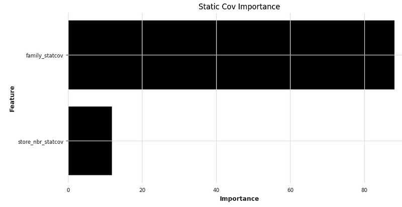

In the TFT model, the attention visualization is done using a technique called multi-head attention. Multi-head attention allows the model to jointly attend to information from different representation subspaces at different positions. The attention weights are learned during training and are used to compute a weighted sum of the input sequence, which is then passed through a non-linear activation function to generate the output.

The attention weights for future predictions can be visualized as well. Figure (F), a graph like the light refraction of a Pyramid, shows the attention weights for the future. The predictions for the immediate future have higher attention weights, and those for far future have lower attention weights.

the explainer.plot_attention(explainability_result, plot_type="all", show_index_as='time')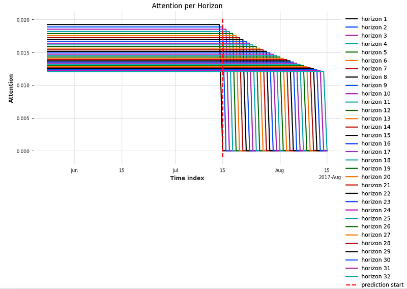

Conclusions

In this chapter, we explained the Temporal Fusion Transformer (TFT) technique. The chapter highlighted four significant aspects of the Temporal Fusion Transformer: Multi-Horizon Forecasting, Interpretability, Temporal Fusion Mechanism, and Transformer Architecture. The chapter demonstrated how to build a global model with covariates. Then it explained how to interpret the model interpretation exhibits of TFT.

Appendix

Because TFT is a neural-network model, it employs the standard neural-network hyperparameters. Here we will understand the concepts of “dropout”, “batch size”, and “epoch”.

Dropout

In a neural network, dropout is a regularization technique used to prevent overfitting and improve the model’s generalization performance. Overfitting occurs when a model fits the training data too closely, resulting in poor performance on new, unseen data.

Dropout works by randomly dropping out (setting to zero) some of the neurons in a layer during training, with a probability specified by the user. This forces the remaining neurons to learn more robust features, as they must compensate for the missing neurons.

During testing, all neurons are used, as the dropped-out neurons are not actually removed from the network. This helps to prevent overfitting, as the model is less likely to rely on any particular set of neurons to make predictions.

The dropout rate, or the probability of dropping out a neuron, is typically set between 0.1 and 0.5. A higher dropout rate can lead to better generalization performance, but may also result in a decrease in model capacity, as some neurons are effectively removed from the network during training.

Batch size

The batch size refers to the number of training examples processed in one forward and backward pass during each iteration of the training process. During training, the neural network is presented with a large number of input examples, each of which is passed through the network to calculate the output. The network’s parameters are then adjusted based on the difference between the predicted output and the actual output, in a process known as backpropagation.

The batch size determines how many input examples are used to update the parameters at each iteration. A larger batch size can provide more reliable estimates of the gradient, which can improve the accuracy and stability of the training process. However, a larger batch size also requires more memory and computational resources, which can be a limitation for certain applications.

I like to use a baking story to explain the concept of batch size in neural networks. Imagine you have a large batch of cookie dough that you want to bake. You can choose to bake the cookies in small batches or large batches. If you bake the cookies in one large batch, the baking time will be unbearably long (lol). You can split the cookies into batches, like 8 or 16 batches. You process a few training examples at a time. This allows for more frequent updates to the model’s parameters, as the gradients are computed and applied after each small batch. It can lead to faster convergence and more frequent weight updates, but it may also introduce more noise in the parameter updates due to the limited sample size.

Epoch

An epoch is a single pass through the entire training dataset. During each epoch, the neural network predicts each example in the training dataset and then updates its weights and biases based on the error between the predicted and actual values.

In the book “Transfer learning for image classification”, I explain the concept of an epoch with a dataset of 1,000 images. During each epoch, the neural network will predict each of the 1,000 images, and then update its weights and biases based on the error between the predicted and actual values. This process is repeated for a fixed number of epochs until the neural network has seen the entire training dataset multiple times.

The number of epochs determines how many times the neural network will see the entire training dataset. If the number of epochs is too low, the neural network may not have enough opportunities to learn the underlying patterns in the data, and may produce inaccurate predictions. On the other hand, if the number of epochs is too high, the neural network may overfit the training data and may produce inaccurate predictions on new, unseen data.

References

• [1] Lim, B., Arik, S.Ö., Loeff, N., & Pfister, T. (2019). Temporal Fusion Transformers for Interpretable Multi-horizon Time Series Forecasting. ArXiv, abs/1912.09363.
• [2] Vaswani, A., Shazeer, N., Parmar, N., Uszkoreit, J., Jones, L., Gomez, A. N., Kaiser, Ł. & Polosukhin, I. (2017). Attention is all you need. Advances in Neural Information Processing Systems (p./pp. 5998–6008).
• [3] Kuo, C. (2023). The Handbook of NLP with Gensim: Leverage topic modeling to uncover hidden patterns, themes, and valuable insights within textual data. Packt Publishing.