Linear Regression for Multi-period Probabilistic Forecasting

Linear regression models, not surprisingly, can do a point estimate for time series. Linear regression models are appealing because they are quick, interpretable, and easy to deploy. It still is a good choice in many organizations. The common type of linear regressions is the autoregressive model, as demonstrated in Automatic ARIMA. However, many real-world use cases demand us to provide the following two: (1) probabilistic forecasts (or called prediction intervals or prediction uncertainty), and (2) multi-period-ahead predictions. How can we extend a linear regression to perform the above two outcomes?

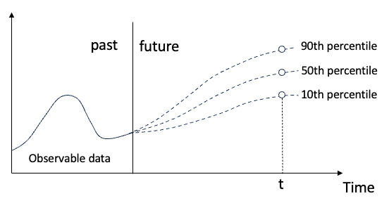
The solution for (1) is to use quantile regression to provide the prediction uncertainty. Figure (A) shows the quantile forecasts. For any future time t, it returns the forecasting samples on the 10th, 50th, and 90th percentile. More quantile samples can be generated if needed. You can go to Chapter 10: “Quantile regression for prediction uncertainty” to learn it.

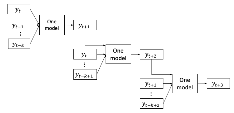
Figure (A): Quantile regression for time series (image by author)

How do we meet (2)? We know a linear regression produces a point prediction, how do we make it multi-period? Maybe one way is to use the same model recursively. We get the one-period prediction from the model as the input to forecast the next period. Then we take the prediction for the second period as the input to forecast the third period. We can iterate through all the periods by using the predictions of the prior periods. This is what the recursive forecasting or iterative forecasting strategy does. Figure (A) shows the model first produces yt+1, then the same model takes yt+1 to produce yt+2, and so on.

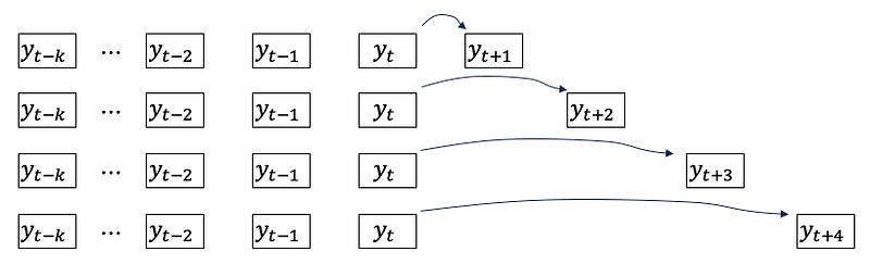
Figure (B): The recursive strategy (image by author)

Another strategy is to build n separate models. Each model produces the forecast for each of the n periods. If we want to predict 10 periods, we will train 10 models and each one to predict a specific step. This is called the direct forecasting strategy. This strategy is shown in Figure (B). You can go to Chapter 11 “A Tutorial on Multi-period Time Series Forecasts” to learn the two strategies.

Figure (C): The direct forecasting strategy (image by author)

Obviously there is no reason to limit the linear regression to univariate time series. Other variables, called covariates, can be added as well. Figure (D) includes other covariates xt and its past p terms.

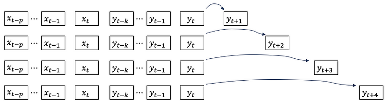
Figure (D): A linear regression with other covariates (image by author)

The linear model seems complex when it needs to perform quantile predictions as shown in Figure (A) and direct forecasting as shown in Figure (D). The good news such a process has been engineered in the Python library for time series called Darts. The Darts library wraps many “scikit-learn” functions so it can leverage the capabilities of “scikit-learn” including the quantile regressor in sklearn. Thus we can focus on the Darts library.

To make your learning easy, we will do this step by step.

The linear regression models of the Darts library.
Start with univariate data for
Include other covariates, then
Include quantile predictions.

The Darts library has its special data format for time series. To make the learning for Darts easier, we covered the data formats of Darts in the previous chapter “Data formats for time series made easy” and you are recommended to reference that chapter. The Python notebook for this chapter is available via this Github link.

Let’s load the data first.

Data

I will use the Walmart dataset on Kaggle.com that contains weekly store sales from 2010–02–05 to 2012–11–01. This dataset contains

Date — the week of sales
Store — the store number
Weekly sales — sales for a store
Holiday flag — whether the week is a special holiday week 1 — Holiday week 0 — Non-holiday week
Temperature — Temperature on the day of sale
Fuel price — Cost of fuel in the region

And two macroeconomic indicators that can affect retail sales: the consumer price index, and the unemployment rate. I will load the dataset as a Pandas data frame.

%matplotlib inline
import pandas as pd
import numpy as np
from matplotlib import pyplot as plt

from google.colab import drive
drive.mount('/content/gdrive')
path = '/content/gdrive/My Drive/data/time_series'
data = pd.read_csv(path + '/walmart.csv', delimiter=",")
data['ds'] = pd.to_datetime(data['Date'], format='%d-%m-%Y')
data.index = data['ds']
data = data.drop('Date', axis=1)
data.head()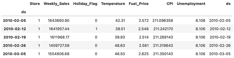

In the chapter “Data formats for time series made easy”, we have learned the special data formats of Darts. The main data class of darts is its TimeSeries class. Darts store the values in an array of shapes (time, dimensions, samples):

Time: The time index, like the 143 weeks in the above example.
Dimensions: The “columns” of multivariate series
Samples: The values for a period. If it is probabilistic predictions like the three samples in Figure (A) for the 10th, 50th, and 90th percentile, there will be three samples.

We will use the function .from_group_dataframe() to load the Walmart store sales. The group ID is “Store”. So the parameter group_cols is “Store”. The time index is the “ds” column.

from darts import TimeSeries
darts_group_df = TimeSeries.from_group_dataframe(data, group_cols='Store', time_col='ds')
print("The number of groups/stores is:", len(darts_group_df))
print("The number of time period is: ", len(darts_group_df[0]))

The number of groups/stores is: 45 The number of periods is: 143

We can list the columns by using the .components function:

darts_group_df[0].components

Index([‘Weekly_Sales’, ‘Holiday_Flag’, ‘Temperature’, ‘Fuel_Price’, ‘CPI’, ‘Unemployment’], dtype=’object’, name=’component’)

To build the model for Store 1 sales, we will just use the data of Store 1. It is “darts_group_df[0]”. We will split it into the training and test data.

store1 = darts_group_df[0]
train = store1[:130]
test = store1[130:]
len(train), len(test) # (130, 13)

Our target series is “Weekly_Sales”. We also can include other covariates. In time series there are two types of covariates: past covariates and future covariates. So the Darts Library follows the same terminology. The past covariates are variables up to the present time of study. And future covariates are observable variables in the future. You may ask how we know future values. Yes, the first reason they are deterministic values such as future holidays. The second reason is they are the predictions from other sources, such as weather forecasts for the next few days. In our case, we will include the “Fuel_price” and “CPI” as the past covariates and “Holiday_flag” as the future covariates. Notice the target and the past covariates in the training data have 130 data points. But the future covariates truly extend to the future and have 143 data points.

target = train['Weekly_Sales'] #130 weeks
past_cov = train[['Fuel_Price','CPI']] # 130 weeks
future_cov = store1['Holiday_Flag'][:143] #143 weeks

Let’s start with univariate data only.

(1) Univariate data only, no covariates

The code below is the basic formulation in the.LinearRegressionMode class of Darts.

from darts.models import LinearRegressionModel
n = 11
model = LinearRegressionModel(
    lags=12,
    multi_models = True # The default
)

Its primary input parameters are:

lags: the number of lagged terms
multi_models: either the direct forecasting strategy or the recursive forecasting strategy for the multi-period-ahead prediction. The default is True, meaning the direct forecasting strategy.

Then we fit the data with the univariate series “target”. We will predict the next n period.

model.fit(target)
pred = model.predict(n)
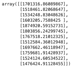
pred.values()

The output is the prediction for the next n periods. Notice the above code already executes the direct forecasting strategy.

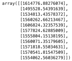
Let’s put the training data, the predicted and the actual values in a plot:

import matplotlib.pyplot as plt
target.plot(label = 'train')
pred.plot(label = 'prediction')
test['Weekly_Sales'][:n].plot(label = 'actual')

The plot is:

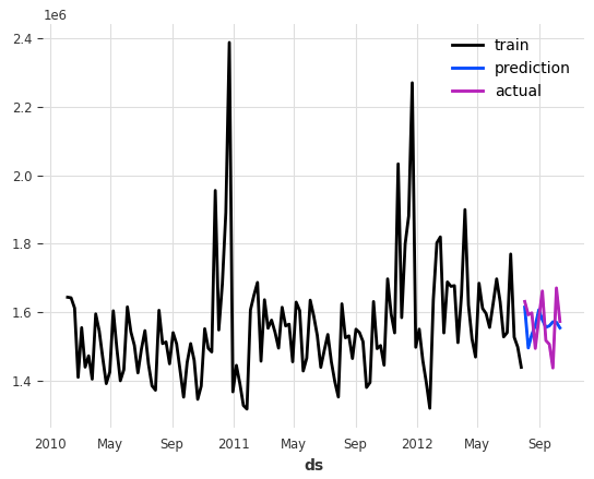
How does the model perform? Let’s use the mean absolute error or the mean absolute percentage error.

from darts.metrics.metrics import mae, mape
print("Mean Absolute Error:", mae(test['Weekly_Sales'][:n], pred))
print("Mean Absolute Percentage Error", mape(test['Weekly_Sales'][:n], pred))

The MAPE is 4.07%:

Mean Absolute Error: 63404.82928050449
Mean Absolute Percentage Error 4.070126403190025

Now let’s add other covariates.

(2) Add past and future covariates

Covariates are additional variables. Darts takes two types of covariates for modeling. One is lags_past_covariates for the lagged past_covariates. The other one is a somewhat confusing name lags_future_covariates for future covariates. “Future covariates” refer to the values of these covariates at future time steps. And “Lagged” values refer to the future covariates from previous time steps. So this means that for the time t + n step in the future, the model considers the values of the covariates at t to t + (n-1) features.

from darts.models import LinearRegressionModel
n = 12
model = LinearRegressionModel(
    lags=12,
    lags_past_covariates=12,
    lags_future_covariates=[0,1,2,3,4,5,6,7,8,9,10,11,12],
    output_chunk_length=12,
)
model.fit(target, past_covariates=past_cov, future_covariates=future_cov)
pred = model.predict(n)
pred.values()

The above parameter output_chunk_length needs more explanation. This is regarding the generation of samples from univariate series. Figure (E) shows samples created from the series y0 to y15. Each sample contains an input chunk and an output chunk. Assume the input chunk length is 5 and the output chunk length is 2. The first sample has y0 — y4 as the input chunk and y5, y6 as the output chunk. The window slides alone the series to create samples until the end of the series.

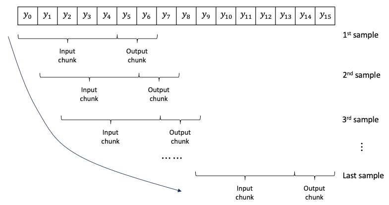
Figure (E): The input chunk and output chunk (image by author)

The output chunk length defines the longest length that can be predicted. We specify it to 12. If we want to predict more than 12, we will receive an error message.

Next, the parameter multi_models specifies the direct forecasting strategy to build multiple separate n models for each of the future n periods. Its default value is True. So here we do not need to specify it.

After modeling and prediction, let’s put the actual and the predicted values together in a plot.

import matplotlib.pyplot as plt
target.plot(label = 'train')
pred.plot(label = 'prediction')
test['Weekly_Sales'][:n].plot(label = 'actual')

The plot looks like this:

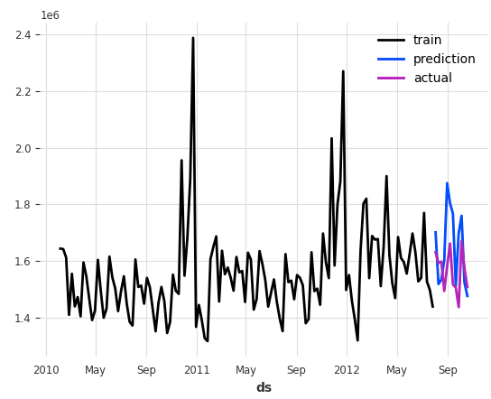
Let’s measure its performance.

print("Mean Absolute Error:", mae(test['Weekly_Sales'][:n], pred))
print("Mean Absolute Percentage Error", mape(test['Weekly_Sales'][:n], pred))

Mean Absolute Error: 119866.3976798996
Mean Absolute Percentage Error 7.738643655822244

Its MAPE is 7.73%, less than the previous model. We could have chosen the previous model. Next, we will learn how to generate quantile forecasts.

(3) Quantile forecasts

The code below adds quantiles=[0.01,0.05,0.50,0.95,0.99]. Because there are 5 samples, we will specify num_samples=5 in .predict().

from darts.models import LinearRegressionModel
n = 12
chunk_length = n
model = LinearRegressionModel(
    lags=12,
    lags_past_covariates=12,
    lags_future_covariates=[0,1,2,3,4,5,6,7,8,9,10,11,12],
    output_chunk_length=chunk_length,
    likelihood = 'quantile', # Can be set to quantile or poisson.
    # If set to quantile, the sklearn.linear_model.QuantileRegressor is used. 
    # Similarly, if set to poisson, the sklearn.linear_model.PoissonRegressor is used.
    quantiles=[0.01, 0.05, 0.50, 0.95,0.99]
)
model.fit(target, past_covariates=past_cov, future_covariates=future_cov)
pred = model.predict(n, num_samples=5)
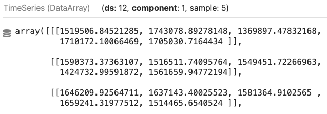
pred

There are five samples for each period. The predictions for each period will be 5 samples instead of one sample. (That’s why the data format of Darts is called the “sample”.)

We will plot the actual values, and the probabilistic forecasts in a plot.

import matplotlib.pyplot as plt
target.plot(label = 'train')
pred.plot(label = 'prediction')
test['Weekly_Sales'][:n].plot(label = 'actual')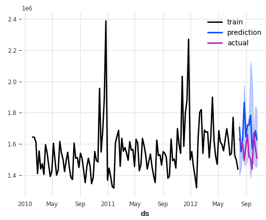

The above predictions come with the light blue area for the probabilistic forecasts.

Conclusions

In this chapter, we learned the linear regression model class of the Darts library. It enables us to build a linear model for multi-period-ahead probabilistic forecasts. We learned the key inputs of the model class including the past and future covariates, and its options for the direct or recursive forecasting strategy for multi-period-ahead predictions. We have also learned how to set up the model for quantile probabilistic forecasts.

This chapter wraps up the modern regression-based time series techniques:

In the next unit, we will study the tree-based modeling techniques: