Tree-based XGB, LightGBM, and CatBoost Models for Multi-period Time Series Probabilistic Forecasting

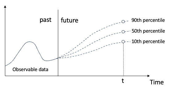
The chapter title covers three essential combinations: “probabilistic forecasting”, “multi-period”, and “tree-based”. This long title refers to the significant predictability that tree-based models can do for time series. First is the “probabilistic forecasting”. Many real-world applications request prediction intervals to manage uncertainty. When we budget for the possible return in a business, we typically want a range of estimates rather than a single value. Quantile predictions provide good solutions. Quantile predictions can inform users of the likelihood of a predicted value, whether it is very likely in the 50th percentile, or very unlikely in the upper 90th percentile as shown in Figure (A).

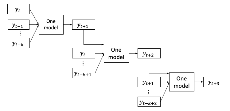
Figure (A): Quantile predictions (image by author)

The second element in the title is multi-period predictions. When you plan for a weekly long vacation and check the weather, you want the weather forecasts for the next 5 days rather than the forecast for only 1 day. We often need forecasts for multiple periods rather than just a point estimate. However, a linear regression or a tree-based algorithm typically provides a point estimate. How do we design the forecasting process to provide multiple periods? Intuitively, if we get the prediction for the next period, maybe we can include it as the input for the same model to get the prediction for the next next period? This solution is popular and is called the recursive forecasting strategy as shown in Figure (B). The recursive forecasting strategy uses the model’s forecasts as inputs for subsequent predictions. The strategy starts with the past values yt to yt-k for the model to predict the one-step-ahead yt+1. Then it incorporates yt+1 and updates other inputs to forecast yt+2. It repeats the process to predict all the subsequent time steps. In the Darts library, you can assign this strategy as well.

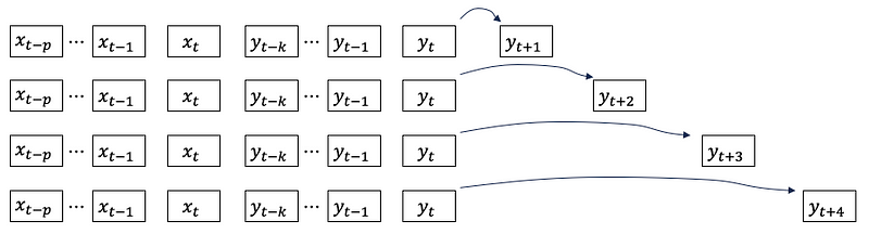
Figure (B): The recursive forecasting strategy for multi-period predictions (image by author)

Let’s think differently. If the goal is to predict n periods ahead, why don’t we build n models separately? Each model will predict each of the next n periods as shown in Figure (A). This is called the direct forecasting strategy. This is the default strategy of the Darts library for all the models included in its library.

Figure (C): The direct forecasting strategy for multi-period predictions (image by author)

Last but not least, let’s discuss the “tree-based” in the chapter title. Tree-based algorithms are supervised learning algorithms. They require a data frame that has rows as samples and columns as features. How does a univariate time series become a data frame? The basic idea is to generate samples from a univariate time series. By doing so we have reorganized a univariate time series to a data frame for modeling. Also, we can create features from the univariate time series.

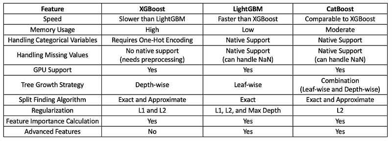
We will introduce the three tree-based models XGBoost (2016), LightGBM (2017), and CatBoost (2018) in three sections, and give a brief description for each algorithm. You may ask about the differences among the three models. I made a table in Figure (C) to highlight the features of the three gradient boost-based algorithms.

Figure (D): The comparisons of XGBoost, LightGBM, and CatBoost (image by author)

This chapter completes the tree-based unit in this book.

A Tutorial on Tree-based Time Series Forecasting
A Tutorial on Multi-period Time Series Forecasts
Tree-based Models XGB, LightGBM, and CatBoost for Multi-period Time Series Probabilistic Forecasting

We will use the Darts library in this chapter. Because time series modeling requires the storage of many features and data, the Darts library has its specific data format. This book dedicated the previous chapter “Time Series Data Formats Made Easy” to explain the strengths of different data formats to contain rich information in time series. Finally, this chapter resembles the previous chapter Linear Regression for Multi-period Probabilistic Forecasting. The two chapters are arranged to assist you in building linear regression and tree-based models in a row for you to select the winning model for your project.

The structure of this chapter is as follows:

The necessary software requirement
Converting a Pandas data to the Dart data format.
XGB
LightGBM
CatBoost

The Python notebook is available for download via this Github link.

Software requirement

The default Darts package does not install Prophet, CatBoost, and LightGBM dependencies, as of version 0.25.0. You need to manually install the Prophet, CatBoost, and LightGBM packages.

CatBoostModel: Install the catboost package (version 1.0.6 or more recent) using the CatBoost install guide
LightGBMModel: Install the lightgbm package (version 3.2.0 or more recent) using the LightGBM install guide

!pip install pandas numpy matplotlib darts lightgbm catboost

Next, we will load the same Walmart store sales data.

Data

I will use the Walmart dataset on Kaggle.com that contains weekly store sales from 2010–02–05 to 2012–11–01. This dataset contains

Date — the week of sales
Store — the store number
Weekly sales — sales for a store
Holiday flag — whether the week is a special holiday week 1 — Holiday week 0 — Non-holiday week
Temperature — Temperature on the day of sale
Fuel price — Cost of fuel in the region

And two macroeconomic indicators that can affect retail sales: the consumer price index, and the unemployment rate. The dataset is loaded as a Pandas data frame.

%matplotlib inline
import pandas as pd
import numpy as np
from matplotlib import pyplot as plt

# Google Colab
from google.colab import drive
drive.mount('/content/gdrive')
path = '/content/gdrive/My Drive/data/time_series'
# https://www.kaggle.com/datasets/yasserh/walmart-dataset

# Load the data
data = pd.read_csv(path + '/walmart.csv', delimiter=",")
data['ds'] = pd.to_datetime(data['Date'], format='%d-%m-%Y')
data.index = data['ds']
data = data.drop('Date', axis=1)
data.head()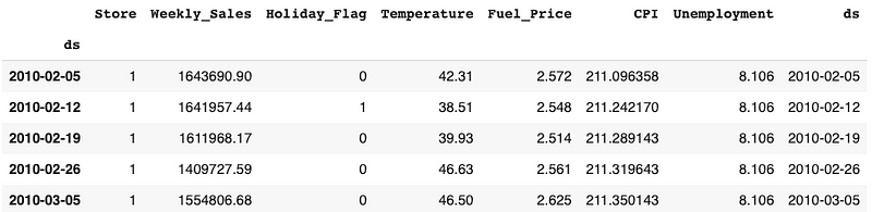

In the chapter “Data formats for time series made easy”, we have learned the special data formats of Darts. The main data class of darts is its “TimeSeries” class. Darts store the values in an array of shapes (time, dimensions, samples):

Time: The time index, like the 143 weeks in the above example.
Dimensions: The “columns” of multivariate series
Samples: The values for a period. If it is probabilistic predictions like the three samples in Figure (A) for the 10th, 50th, and 90th percentile, there will be three samples.

We will use the function .from_group_dataframe() to load the Walmart store sales. The group ID is “Store”. So the parameter group_cols is “Store”. The time index is the “ds” column.

from darts import TimeSeries
darts_group_df = TimeSeries.from_group_dataframe(data, group_cols='Store', time_col='ds')
print("The number of groups/stores is:", len(darts_group_df))
print("The number of time period is: ", len(darts_group_df[0]))

The number of groups/stores is: 45
The number of periods is: 143

We can list the columns by using the.components function:

darts_group_df[0].components

Index([‘Weekly_Sales’, ‘Holiday_Flag’, ‘Temperature’, ‘Fuel_Price’, ‘CPI’, ‘Unemployment’], dtype=’object’, name=’component’)

To build the model for Store 1 sales, we will just use the data of Store 1. It is “darts_group_df[0]”. We will split it into the training and test data.

store1 = darts_group_df[0]
train = store1[:130]
test = store1[130:]
len(train), len(test) # (130, 13)

Our target series is “Weekly_Sales”. We also can include other covariates. In time series there are two types of covariates: past covariates and future covariates. So the Darts Library follows the same terminology. The past covariates are variables up to the present time of study. And future covariates are observable variables in the future. You may ask how we know future values. Yes, the first reason they are deterministic values such as future holidays. The second reason is they are the predictions from other sources, such as weather forecasts for the next few days. In our case, we will include the “Fuel_price” and “CPI” as the past covariates and “Holiday_flag” as the future covariates. Notice the target and the past covariates in the training data have 130 data points. But the future covariates truly extend to the future and have 143 data points.

target = train['Weekly_Sales']
past_cov = train[['Fuel_Price','CPI']]
future_cov = store1['Holiday_Flag'][:143]

Let’s start with univariate data only.

XGB

XGBoost (Extreme Gradient Boosting) is widely used for supervised learning tasks such as classification and regression and is known for its efficiency, scalability, and accuracy. Its most salient feature is it includes L1 and L2 regularization techniques to prevent overfitting. Regularization penalties are applied to the tree weights, leaf node values, and feature importance scores, helping to improve generalization performance. Another feature is its support for parallel and distributed computing, enabling efficient training on multi-core CPUs and distributed computing frameworks such as Apache Spark and Dask. This scalability makes it suitable for handling large datasets. Other than that, it inherits the gradient-boosting framework, which involves the sequential training of an ensemble of decision trees. Each tree is trained to correct the errors made by the previous models, with the overall goal of minimizing a specified loss function.

The following code is the standard modeling syntax of Darts.

from darts.models import XGBModel
n = 12
chunk_length = n
model = XGBModel(
    lags=12,
    lags_past_covariates=12,
    lags_future_covariates=[0,1,2,3,4,5],
    output_chunk_length=12,
    Multi_models = True # optional
    verbose=-1
)
model.fit(target, past_covariates=past_cov, future_covariates=future_cov)
pred = model.predict(n)
pred

The “target” in fit() is the target series for modeling. The model requires “lags” for the number of lagged values yt, yt-1, yt-2, …, yt-12. The model also lets you specify other covariates. In time series modeling there are two broad types of covariates, namely, the past covariates and future covariates. Darts follow this convention. The lags_past_covariates refers to the lagged past covariates like xt, xt-1, …, xt-12. The somewhat confusing name lags_future_covariates refers to future covariates. “Future covariates” mean the values of these covariates at future time steps, and “Lagged” values mean the future covariates from previous time steps. This means that for the time t + n step in the future, the model considers the values of the covariates at t to t + (n-1) features.

Notice the multi_models parameter is set to True. It tells the model to use either the direct forecasting strategy or the recursive forecasting strategy for multi-period predictions. The default is True, meaning the direct forecasting strategy.

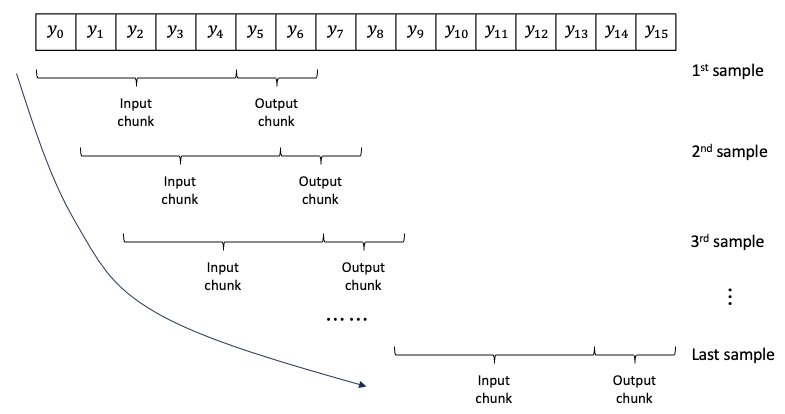
One more parameters are the input chunk length and the output chunk length. This is regarding the generation of samples from univariate series. Figure (E) shows samples created from the series y0 to y15. Each sample contains an input chunk and an output chunk. Assume the input chunk length is 5 and the output chunk length is 2. The first sample has y0 — y4 as the input chunk and y5, y6 as the output chunk. The window slides alone the series to create samples until the end of the series. The output chunk length defines the longest length that can be predicted. We specify it to 12. If we want to predict more than 12, we will receive an error message.

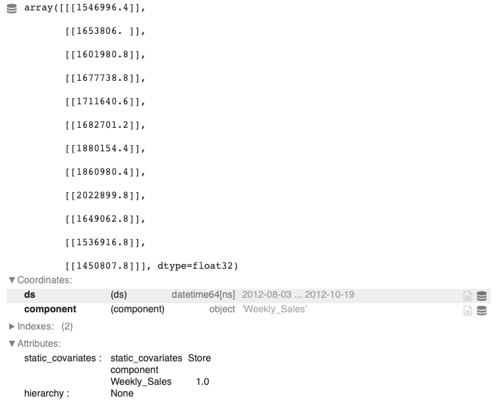
Figure (E): The input chunk and output chunk (image by author)

The outputs are stored in the Dart data array:

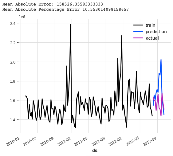
We will plot the actual and the predicted values. We make this in a function for repeating use.

def plotit():
  import matplotlib.pyplot as plt
  target.plot(label = 'train')
  pred.plot(label = 'prediction')
  test['Weekly_Sales'][:n].plot(label = 'actual')

  from darts.metrics.metrics import mae, mape
  print("Mean Absolute Error:", mae(test['Weekly_Sales'][:n], pred))
  print("Mean Absolute Percentage Error", mape(test['Weekly_Sales'][:n], pred))

plotit()

The MAPE is 10.55%.

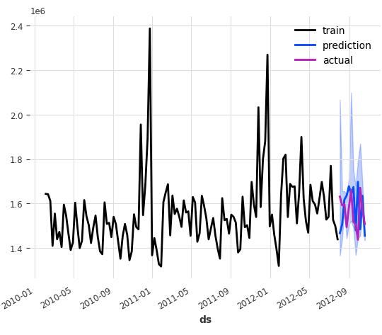
Let’s add the quantile predictions. We will ask the model to create 5 quantiles.

from darts.models import XGBModel
n = 12
chunk_length = n
model = XGBModel(
    lags=12,
    lags_past_covariates=12,
    lags_future_covariates=[0,1,2,3,4,5,6,7,8,9,10,11,12],
    output_chunk_length=chunk_length,
    likelihood = 'quantile', # Can be set to quantile or poisson.
    # If set to quantile, the sklearn.linear_model.QuantileRegressor is used.
    # Similarly, if set to poisson, the sklearn.linear_model.PoissonRegressor is used.
    quantiles=[0.01, 0.05, 0.50, 0.95,0.99]
)
model.fit(target, past_covariates=past_cov, future_covariates=future_cov)
pred = model.predict(n, num_samples=5)
pred

There are 5 samples in each prediction because we generate 5 quantile values.

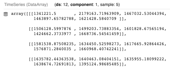
We can plot the actual values and the quantile predictions.

def plotQuantile():
    import matplotlib.pyplot as plt
    target.plot(label = 'train')
    pred.plot(label = 'prediction')
    test['Weekly_Sales'][:n].plot(label = 'actual')

plotQuantile()

The quantile forecasts are:

You may find it very easy to build the model and provide predictions. Let’s continue to build lightGBM models.

LightGBM

Didn’t we build a lightgbm model in the previous chapter “A Tutorial on Tree-based Time Series Forecasting”? Indeed! The difference is that here we will use the Darts library to build lightgbm models. The data format in the previous chapter is a Pandas data frame, and here is a Darts data objective. Let’s still explain what LightGBM is.

LightGBM (Light Gradient Boosting Machine) is designed for efficient and scalable training of gradient-boosting decision tree models. LightGBM has gained popularity for its speed, memory efficiency, and accuracy. Its unique feature is its leaf-wise growth strategy instead of the traditional level-wise strategy used in other gradient-boosting implementations. This strategy chooses the leaf node that will minimize the loss most effectively, resulting in faster training times. Other than that, it still implements the gradient boosting algorithm.

from darts.models import LightGBMModel
n = 12
model = LightGBMModel(
    lags=12,
    lags_past_covariates=12,
    lags_future_covariates=[0,1,2,3,4,5],
    output_chunk_length=12,
    verbose=-1
)
model.fit(target, past_covariates=past_cov, future_covariates=future_cov)
pred = model.predict(n)
pred.values()

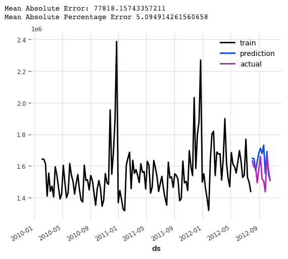
The above code is similar to that in XGB so we do not highlight more. Let’s plot it and get performance metrics:

plotit()

The MAPE is 5.09%.

Now let’s include the quantile predictions.

n = 12
chunk_length = n
model = LightGBMModel(
    lags=12,
    lags_past_covariates=12,
    lags_future_covariates=[0,1,2,3,4,5,6,7,8,9,10,11,12],
    output_chunk_length=chunk_length,
    likelihood = 'quantile', # Can be set to quantile or poisson.
    # If set to quantile, the sklearn.linear_model.QuantileRegressor is used.
    # Similarly, if set to poisson, the sklearn.linear_model.PoissonRegressor is used.
    quantiles=[0.01, 0.05, 0.50, 0.95,0.99]
)
model.fit(target, past_covariates=past_cov, future_covariates=future_cov)
pred = model.predict(n, num_samples=5)
pred

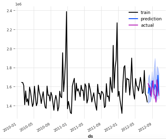
We can plot the quantile forecasts.

plotQuantile()

The quantile forecasts are:

Nice. We have two models built already. Let’s build CatBoost models.

CatBoost

CatBoost stands for “Category Boosting”. It is specifically designed to handle categorical features efficiently, making it well-suited for a wide range of classification and regression tasks. It can handle categorical features directly without the need for pre-processing such as one-hot encoding. It uses a novel algorithm called Ordered Boosting, which efficiently handles categorical variables by finding the optimal split points based on the statistical properties of the categories. Other than that, it still inherits the implementation of gradient boosting in building an ensemble of decision trees sequentially. Each tree is trained to minimize the error of the previous model. It uses a gradient descent optimization algorithm to find the optimal parameters.

from darts.models import CatBoostModel
n = 12
chunk_length = n
model = CatBoostModel(
    lags=12,
    lags_past_covariates=12,
    lags_future_covariates=[0,1,2,3,4,5],
    output_chunk_length=12,
    verbose=-1
)
model.fit(target, past_covariates=past_cov, future_covariates=future_cov)
pred = model.predict(n)
pred

You may find that you just replace the code with the CatBoostModel and everything else remains the same.

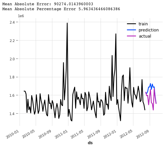
Let’s plot the outcome:

plotit()

The MAPE is 5.96%.

Let’s include the quantile predictions in the model.

n = 12
chunk_length = n
model = CatBoostModel(
    lags=12,
    lags_past_covariates=12,
    lags_future_covariates=[0,1,2,3,4,5,6,7,8,9,10,11,12],
    output_chunk_length=chunk_length,
    likelihood = 'quantile', # Can be set to quantile or poisson.
    # If set to quantile, the sklearn.linear_model.QuantileRegressor is used.
    # Similarly, if set to poisson, the sklearn.linear_model.PoissonRegressor is used.
    quantiles=[0.01, 0.05, 0.50, 0.95,0.99]
)
model.fit(target, past_covariates=past_cov, future_covariates=future_cov)
pred = model.predict(n, num_samples=5)
pred

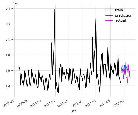
We can plot the quantile predictions.

plotQuantile()

The plot is:

Conclusions

In this chapter, we have used the Darts library to build three popular tree-based time series models. We emphasized the use cases of multi-period forecasts and prediction uncertainty. When next time you need to build time series models to provide multi-period predictions and forecasting uncertainty, you are recommended to build the three tree-based models, together with the linear regression model in the chapter Linear Regression for Multi-period Probabilistic Forecasting to find a winning model.

This chapter wraps up the series on modern techniques for tree-based time series models:

In the next chapter, we will start the series on deep-learning-based time series models.

The Progression of Time Series Modeling Techniques
DeepAR for RNN/LSTM
Application — Probabilistic Predictions for stock prices
Temporal Convolutional Network Time Series Probabilistic Forecasts

References

(XGB) Chen, T., & Guestrin, C. (2016). XGBoost: A Scalable Tree Boosting System. In Proceedings of the 22nd ACM SIGKDD International Conference on Knowledge Discovery and Data Mining (pp. 785–794). ACM. [Link](https://dl.acm.org/doi/10.1145/2939672.2939785)
(LightGBM) Ke, G., Meng, Q., Finley, T., Wang, T., Chen, W., Ma, W., … & Li, Q. (2017). LightGBM: A Highly Efficient Gradient Boosting Decision Tree. In Advances in Neural Information Processing Systems (pp. 3146–3154).(https://proceedings.neurips.cc/paper/2017/file/6449f44a102fde848669bdd9eb6b76fa-Paper.pdf)
(CatBoost) Prokhorenkova, L., Gusev, G., Vorobev, A., Dorogush, A. V., & Gulin, A. (2018). CatBoost: unbiased boosting with categorical features. In Advances in Neural Information Processing Systems (pp. 6638–6648). (https://proceedings.neurips.cc/paper/2018/file/0d4724e4525b451dae9f6cb39983e6cd-Paper.pdf)