Credit Risk Modelling in Python

Introduction

Credit risk modelling is a crucial aspect of the BFSI industry, enabling lenders to assess the probability of borrowers defaulting on loans. We all know what happens to financial institutions profitability and even survival, when loans go rogue!

In this blog, we will explore how to build a credit risk model using Python. We’ll discuss the dataset, try to address the challenge of imbalanced data, preprocess the data, train a logistic regression model, and evaluate its performance. Let’s dive in!

Dataset Overview

The original data used in this exercise comes from publicly available data from LendingClub.com, a website that connects borrowers and investors over the Internet.

Variables used in the Data Dependent Variable — ‘not.fully.paid’: a binary variable indicating that the loan was not paid back in full, i.e, (the borrower either defaulted or the loan was “charged off,” meaning the borrower was deemed unlikely to ever pay it back).

Independent Variables 1) credit.policy: 1 if the customer meets the credit underwriting criteria of LendingClub.com, and 0 otherwise.

2) purpose: The purpose of the loan (takes values “credit_card”, “debt_consolidation”, “educational”, “major_purchase”, etc).

3) int.rate: The interest rate of the loan, as a proportion (a rate of 11% would be stored as 0.11). Borrowers judged by LendingClub.com to be more risky are assigned higher interest rates.

4) installment: The monthly installments ($) owed by the borrower if the loan is funded.

5) log.annual.inc: The natural log of the self-reported annual income of the borrower.

6) dti: The debt-to-income ratio of the borrower (amount of debt divided by annual income).

7) fico: The FICO credit score of the borrower.

8) days.with.cr.line: The number of days the borrower has had a credit line.

9) revol.bal: The borrower’s revolving balance (amount unpaid at the end of the credit card billing cycle).

10) revol.util: The borrower’s revolving line utilization rate (the amount of the credit line used relative to total credit available).

12) inq.last.6mths: The borrower’s number of inquiries by creditors in the last 6 months.

13) delinq.2yrs: The number of times the borrower had been 30+ days past due on a payment in the past 2 years.

14) pub.rec: The borrower’s number of derogatory public records (bankruptcy filings, tax liens, or judgments).

Let’s begin by loading the required libraries and the data.

# Import required libraries
import pandas as pd
import numpy as np
import matplotlib.pyplot as plt
import seaborn as sns
%matplotlib inline

# Import necessary modules
from sklearn.linear_model import LogisticRegression 
from sklearn.model_selection import train_test_split  
from sklearn.metrics import confusion_matrix, classification_report
from sklearn.metrics import roc_auc_score

# Load data
df = pd.read_csv("loansdata.csv")
print(df.shape)

The dataset contains 9578 rows and 14 columns. Always good to just have a look at the dataset, isn’t it? We can do that easily with the df.head() function which produces the following output.

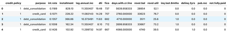
So we have our first glimpse of the data, and before getting into the modelling stage, let’s look at the summary statistics of the variables we have.

The df.describe() function will generate descriptive statistics of the numerical columns. You can add the transpose()utility to switch the rows and columns, making it easier to read and interpret, with columns representing each statistic and rows corresponding to each numerical feature.

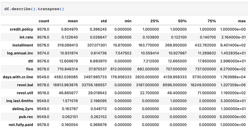
We could embark on an epic journey of detailed exploratory data analysis, venturing into the depths of every variable. However, to keep things snappy and concise, let’s set our sights on the star of the show: the target variable, `not.fully.paid`.

Glancing at the output above, we notice that this mischievous variable plays a binary game, with values of 0 and 1. Ah, the mean value! It stands before us like a secret code, revealing that a mere 16% of the records dared to defy convention and didn’t fully pay back their loans. Quite the rebellious bunch!

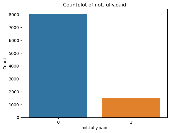
Let’s examine this visually with the code below, that displays the count of occurrences for each unique value of ‘not.fully.paid’ in the dataset.

# Create a countplot of the target variable
sns.countplot(data=df, x='not.fully.paid')

# Set the plot title and axes labels
plt.title("Countplot of not.fully.paid")
plt.xlabel("not.fully.paid")
plt.ylabel("Count")
# Show the plot
plt.show()

Output:

Clearly, we have an imbalanced dataset.

Preparing Data for Modelling

We’ve taken our first steps into the realm of data analysis, and now it’s time to prepare our data for the mighty modeling stage! But before we proceed, we need to shine a light on the shadows of missing values lurking within our dataset.

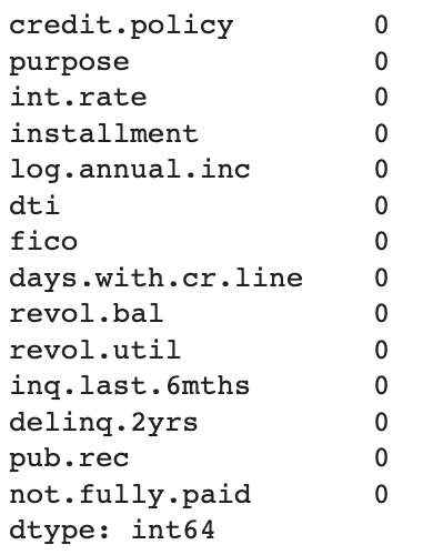
The code below performs the task and generates the number of missing values per variable.

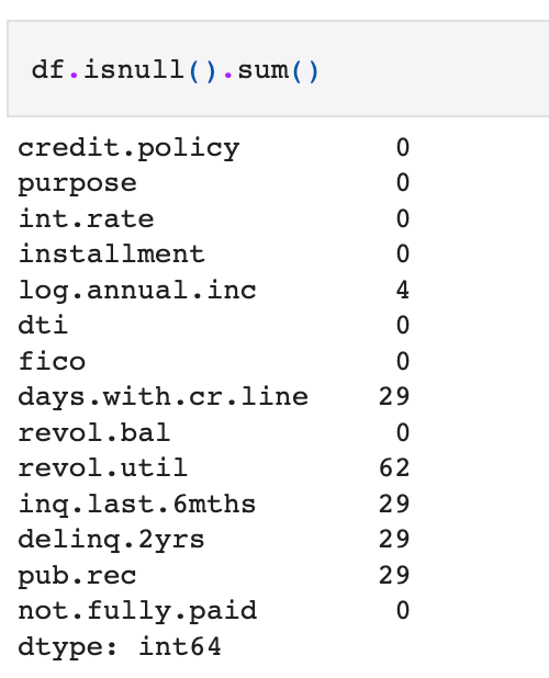
So we can clearly see variables with missing values. Let’s do missing values treatment through median imputation. Of-course, there are other ways also to treat missing values, but that’s for some other day(or blog)!

columns_with_missing = ['days.with.cr.line', 'revol.util', 'inq.last.6mths','delinq.2yrs', 'pub.rec', 'log.annual.inc']

# Replace missing values with median in specified columns
for column in columns_with_missing:
    median = df[column].median()
    df[column].fillna(median, inplace=True)
# Check for the changes 
df.isnull().sum()

Output:

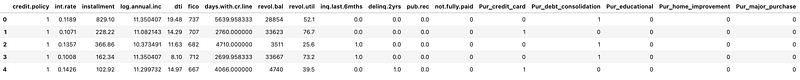
So the missing value transformation is done, and the next transformation needed is to convert the categorical variable, purpose into numerical variables through a technique called one hot encoding.

df = pd.get_dummies(df, columns=['purpose'], drop_first=True, prefix='Pur')
df.head()

Output:

Scaling the predictor variables

We now have our variables ready, and the next step is to scale the predictor variables. Scaling helps us level the playing field and ensures that all predictors have a similar range of values. It’s like bringing everyone to the same height so no one overshadows the others!

The code below performs this task.

target_column = ['not.fully.paid'] 
predictors = list(set(list(df.columns))-set(target_column))
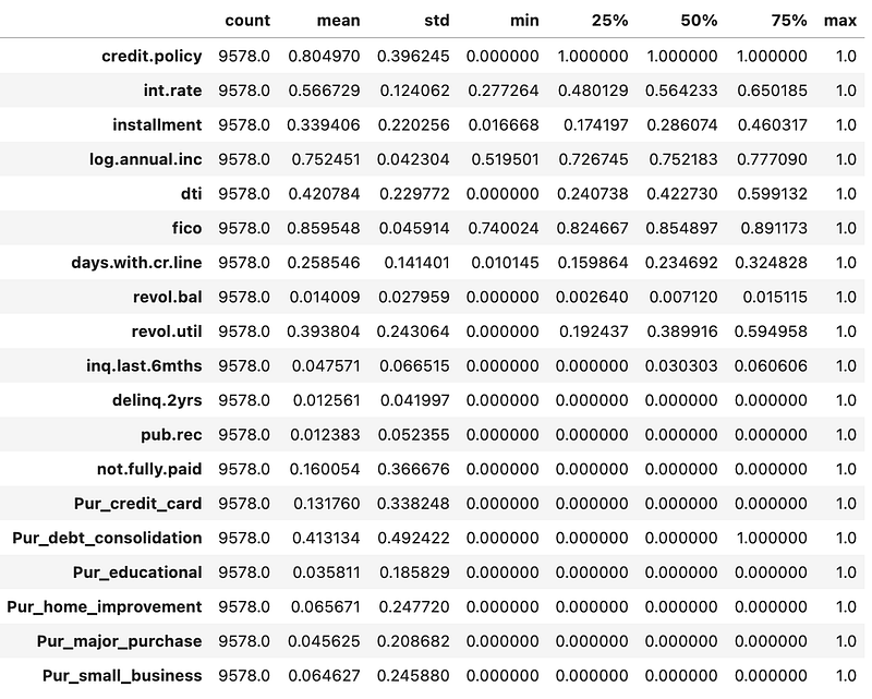
df[predictors] = df[predictors]/df[predictors].max()
df.describe().transpose()

The output below shows that now all the independent variables are scaled between 0 and 1.

Create train and test set arrays

In this code snippet, we’re getting ready to train our machine learning model by splitting our data into training and testing sets. This is called the holdout-validation approach to model evaluation. There are other techniques as well, such as the variants of cross validation, but we’ll be using the train/ test split approach.

In short, we gather our features from the dataset and store them in X, while assigning the target variable to y. To ensure a thorough training and fair testing, we split the data into training and testing sets using the train_test_split function. By displaying the shapes of the training and testing sets, we can verify the number of samples and features in each set, ensuring everything is set for our model's grand performance!

X = df[predictors].values
y = df[target_column].values

X_train, X_test, y_train, y_test = train_test_split(X, y, test_size=0.30, random_state=100)
print(X_train.shape); print(X_test.shape)

Output:

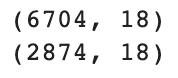
The training and test data has 6704 and 2874 rows, respectively.

Model Training and Evaluation

With the data ready, we’ll now train a logistic regression model using the training data. The logistic regression algorithm is widely used for credit risk modelling due to its interpretability and ability to handle binary classification problems. In real life scenario, often logistic regression is considered as a baseline model, which sets the target to improve upon for other machine learning algorithms.

After training the model, we’ll evaluate its performance on both the training and testing sets. We’ll use classification metrics such as the confusion matrix, classification report, and AUC score to assess the model’s effectiveness.

logreg = LogisticRegression()
logreg.fit(X_train, y_train)

predict_train = logreg.predict(X_train)
predict_test = logreg.predict(X_test)
print(confusion_matrix(y_train,predict_train))
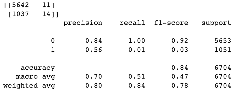
print(classification_report(y_train,predict_train))

Output:

Let’s also look at the model performance on the test dataset.

print(confusion_matrix(y_test,predict_test))
print(classification_report(y_test,predict_test))

Output:

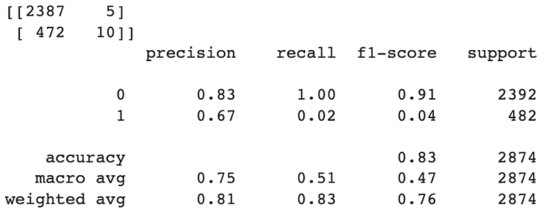
The above output reveals an intriguing revelation about our model’s performance. It seems to excel at predicting non-defaulters, those ideal customers who dutifully pay back their loans. However, when it comes to predicting defaulters, our model falls a bit short of greatness.

Now, hold your excitement for a moment! Don’t be deceived by the seemingly impressive accuracy scores of 84% and 83% on the training and test sets, respectively. Let me drop a truth bomb on you: accuracy is not the best metric to evaluate models dealing with imbalanced data, just like our current scenario.

Here’s the kicker: the bank or financial institution’s primary concern lies in improving the predictability of defaulting customers (those daring souls represented by the number 1 in the `not.fully.paid` variable). They want to sharpen their crystal ball to identify potential defaulters accurately.

So, if not accuracy than what should be the evaluation metric?. Recall, F-1 score and AUC Score are often used in such cases, and we will look at these in the next section where we try to handle imbalance within the dataset.

Handling Imbalance with Class Weights

To address the class imbalance, we can assign class weights to provide a balanced perspective to the model. This can be done by passing the weights to the class_weight argument within the LogisticRegression module as shown in the code below.

# dictionary of class weights
weight_dict = {0:1.19, 1:6.25}

# define the model
logreg2 = LogisticRegression(random_state=10, class_weight=weight_dict)

# fit the model
logreg2.fit(X_train,y_train)

By assigning higher weights to the minority class, we can give it more influence during training. Note that these weights are chosen arbitrarily (with little use of division), and you can choose any other combination as well.

We’ll then train and evaluate a logistic regression model with these custom class weights to observe its impact on performance.

predict_train = logreg2.predict(X_train)
print(confusion_matrix(y_train,predict_train))
print(classification_report(y_train,predict_train))
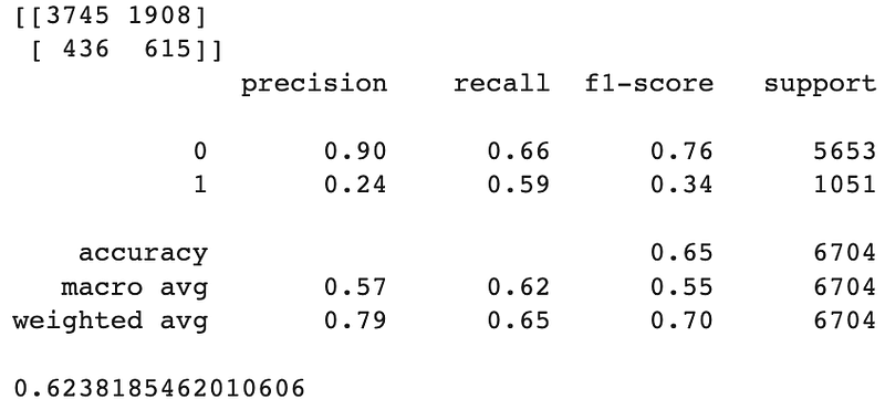
print(roc_auc_score(y_train,predict_train))

Output:

Let’s evaluate the model on test dataset.

predict_test = logreg2.predict(X_test)
print(confusion_matrix(y_test,predict_test))
print(classification_report(y_test,predict_test))
print(roc_auc_score(y_test,predict_test))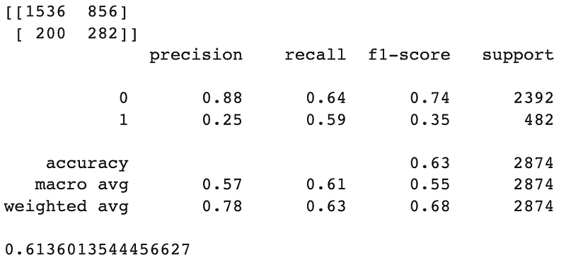

We can clearly observe the notable improvement in the results mentioned above. The recall metric on the test dataset has skyrocketed from a mere 2% to a remarkable 59%, indicating a substantial enhancement in its ability to correctly identify positive cases. Additionally, the AUC score, a measure of overall model performance, has shown promising progress, increasing from 0.5 to 0.61.

Although we have not yet achieved perfection, these advancements serve as a solid baseline for our model’s performance. Moving forward, our objective will be to surpass these results by implementing more sophisticated algorithms and strategies, aiming for even higher metrics. The journey to an impeccable credit risk model continues!

Conclusion

In this blog post, we explored credit risk modelling using Python. We discussed the dataset, implemented preprocessing technique, and addressed the challenge of imbalanced data. We trained a logistic regression model, evaluated its performance, and investigated the impact of using custom class weights.

Next Steps

Our journey doesn’t end here! There are exciting paths to follow and improvements to be made. Listed below are some next steps and suggestions to enhance our model’s performance:

1. Selecting Better Weight Combinations: We can fine-tune the class weights to find an even more effective combination. By experimenting with different weights, we can strike a balance that gives proper consideration to both the minority and majority classes. It’s like finding the perfect recipe for success!

2. Unleashing the Power of Feature Engineering: We can take our model to the next level by applying some feature engineering wizardry. This involves exploring the relationships between variables, identifying correlations, and removing any redundant or highly correlated features. It’s like decluttering our dataset and unleashing the hidden potential within!

3. Embracing Imbalance-Busting Techniques: To conquer the challenges of class imbalance, we can employ powerful techniques like SMOTE (Synthetic Minority Over-sampling Technique). SMOTE creates synthetic samples of the minority class, boosting its representation in the dataset.

4. Unleashing the Beasts: Random Forest, XG Boost, and Deep Neural Nets: Now, it’s time to call upon the heavyweights of the machine learning realm. These mighty algorithms possess extraordinary predictive powers and can handle complex relationships within the data. By exploring these advanced models, we may uncover even greater accuracy and predictive performance.

Remember, fellow science enthusiasts, our quest for the perfect credit risk model continues. As we embark on these next steps, let us embrace the thrill of experimentation and innovation. The possibilities are endless, and the rewards are great. Onward we march, seeking the pinnacle of model performance and the realm of exceptional risk assessment!

If you want to read more on this credit risk data, you can check this link here.

If you’re interested in statistics, data science and machine learning, you’ll like these blogs:

You can also connect with me on LinkedIn.

Good luck!