Advanced Mapping with Stata: OpenStreetMap (OSM) and QGIS

In this guide, we will learn how to import OpenStreetMap (OSM) data in Stata via QGIS which allows us to create extremely detailed choropleth maps from several spatial layers:

The above three cities have been my home in the past four decades, so this guide is a tribute to them! Please feel free to use this guide on any city or location of your choice.

This is the third installment in the Stata maps series and opens up Stata for any type of mapping allowing us to move towards more complex spatial analysis. This guide is recommended for more advanced users who are already familiar with spmaps, tmaps in Stata. If not, then I highly recommend the first map guide which introduces spmap, and the second map guide where we learn to reprograms maps. Most of this guide builds on the second one.

Preamble

Like other guides, a basic knowledge of Stata is assumed. In order to make the graphs exactly as they are shown here, several additional item are required:

In order to make the graphs exactly as they are shown here, install the schemepack suite (more info in the Scheme guide and on GitHub):

ssc install schemepack, replace

Set the schemes to one of the white background one for a clean look:

set scheme white_tableau, perm

Install Ben Jann’s colorpalette package (more on colors in Guide 2 and the Color guide)

ssc install palettes, replace 
ssc install colrspace, replace

Set default graph font to Arial Narrow (see the Font guide on customizing fonts)

graph set window fontface "Arial Narrow"

For workflow management, I use the following folder structure to organize the files, and paths refer to subfolders relative to the root folder:

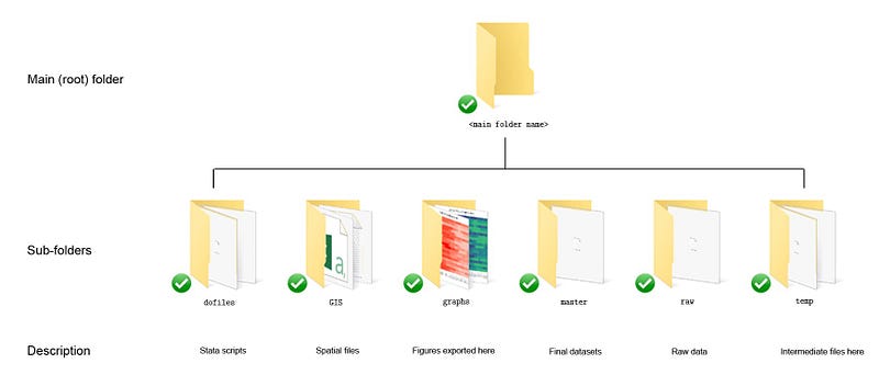
Using folders to organize files is important since files multiply quickly. See Guide 1 for a discussion on this. For this guide, I have dumped all my files in the ./GIS/qgis folder. But whatever folder you use, please make sure you know its path since we will use it later in Stata.

Get the additional packages for maps:

ssc install shp2dta, replace  // shapefiles to dta. For v14 or below

If you are using Stata 14 or earlier then the built-in Stata command spshape2dta command that comes with v15 and higher will need to be replaced by shp2dta. I already discuss this in detail in the first map guide so it won’t be repeated here. Please report errors or workarounds if you come across problems with this guide.

Part I: Extract OSM layers via QGIS

The very first step is to install QGIS. QGIS is an open-source software for spatial data. It also has a unique advantage over the more commercial ArcGIS, in that, it allows one to export OpenStreetMap (OSM) layers as shapefiles:

Once you install the software, you can open an empty project by clicking on either of the two icons highlighted below:

Next, go in the plugins window and search and install QuickOSM:

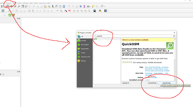
QuickOSM accesses OSM with their API. If you are familiar with APIs and how to extract data from them, you can also do all of this directly as well. But then you are already fairly advanced enough and probably don’t need this guide!

Next step, we need to load OSM in QGIS. This can be done using the Layer menu. Here we click on Add Layer, and within this we click on “Add XYZ Layer”:

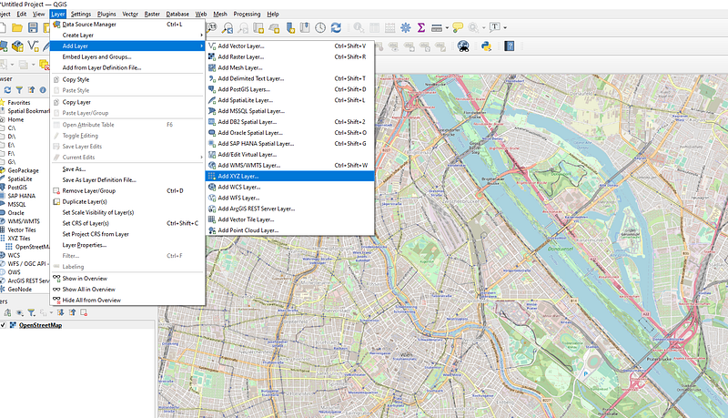
Note that (just as an extra piece of information) in QGIS shapefiles are referred to as Vector Layers (first option in the Add Layer menu).

Here select OpenStreetMap and click Add:

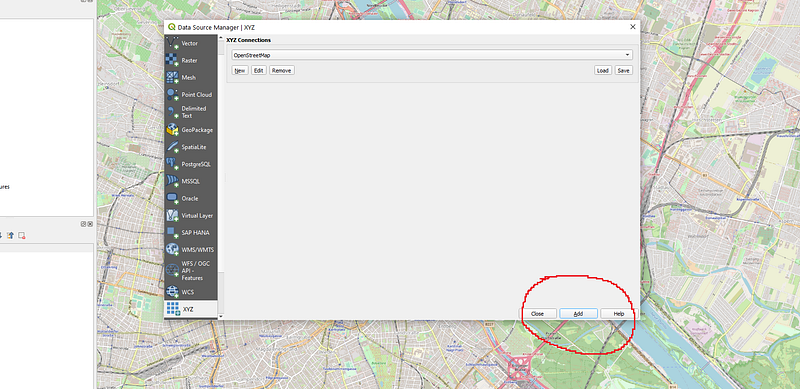
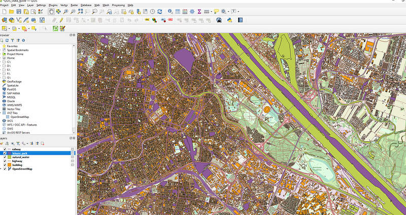
A global map will pop in your QGIS interface window. Here zoom to the location that you want to map. Also be careful of the zoom extent. The more zoomed out your are, the more data needs to be loaded. This also depends on which layers you want to extract. For major cities, this implies a lot of data! I have selected Vienna (my current place of residence) as my choice of the map I want to extract. Please feel free to use any other location. Also save the QGIS file in case the software crashes at some point.

In the OSM layer, get the zoom level and map extent exactly as how you want to export them. Once you have your preferred layout, don’t touch this layer. We will restrict out data download and layer exports to what we see on screen. There are other methods as well but we will stick to this one in this guide.

Get the layers

Now we need to use the QuickOSM plug menu we installed earlier. It can be accessed either from the Vector menu or one can also click on the green icon that is in the taskbar:

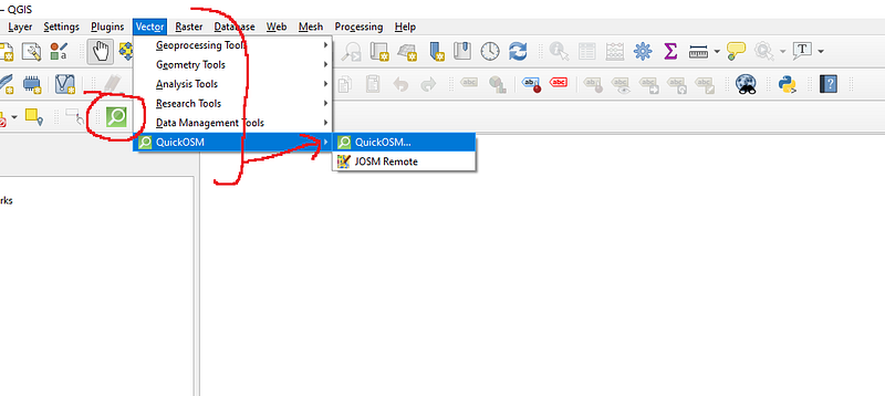
Once you click the QuickOSM icon, this menu pops up:

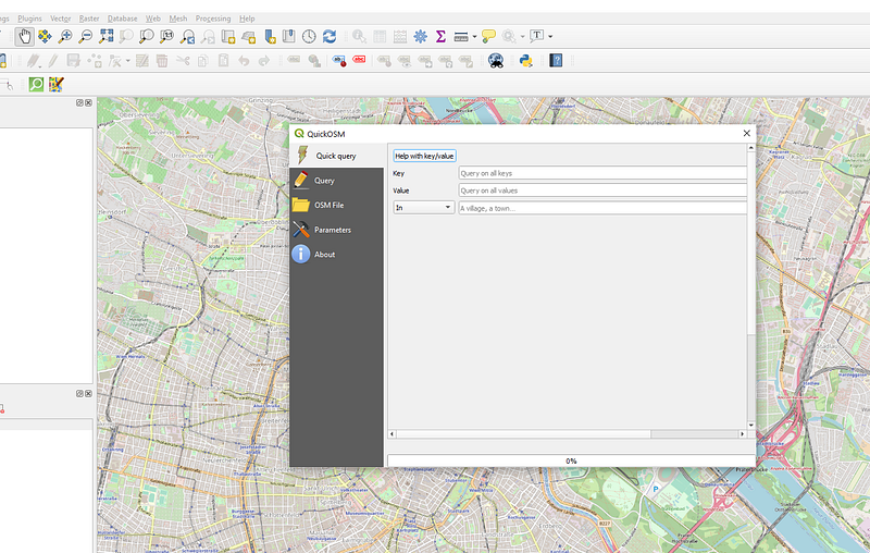
As you can see from the screenshot above, we need to fill in three fields. The first one is the Key. Key in OSM describes the overarching layer category. In OSM these are referred to as Map Features which are listed on this website:

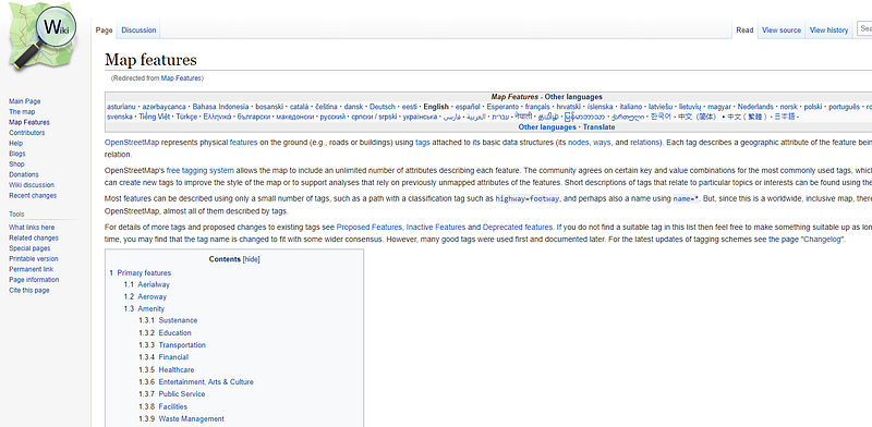
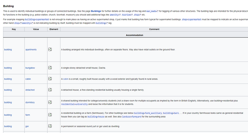
https://wiki.openstreetmap.org/wiki/Map_features

In the above website, one can look at the main categories and the subcategories. The main categories go in the “Key” field, while the sub-categories go in the second “Value” field. For example “building” is a key category. If you type it, QuickOSM will also auto complete it. The dropdown menu can also be used but it does not feature all the possible options:

Typing in “building” means that we want to load everything that is labeled as building regardless of their sub-category type (residential, commercial, industrial etc). In the “In” drop down menu, click on “Canvas Extent” since we want to extract from the map that is showing in the background. Once these fields are filled, click on “Run query”. Extracting layers from OSM might take a while since they depend on your internet speed and the amount of data you want to load. Once this is done, new temporary layers, referred to as “scratch” layers in QGIS, will be added in the layer pane on the left-hand side. GIS layers are of three types: polygons, lines, and points. Since we know that buildings are coded as polygons, the line and point layers basically contain either some unusual information, they are errors, or they are just badly coded points. Right click on the layer and remove these.

If we turn off the base OSM map by unchecking the small box, we are left with the building layer only:

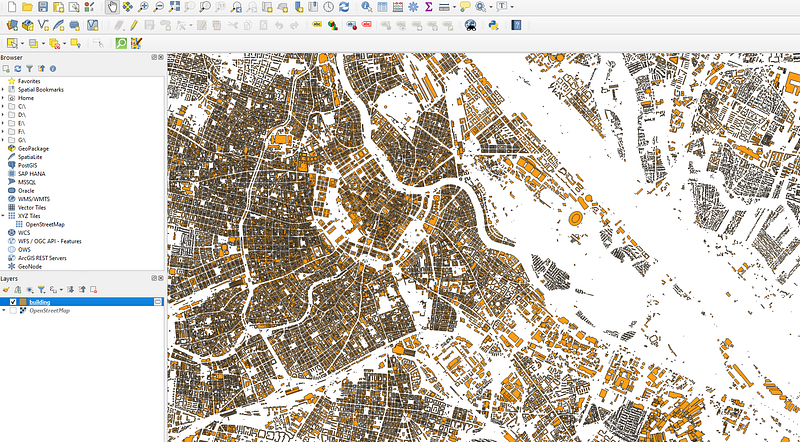
If you want to learn more about this layer, you can right click on the layer icon and look at the attributes. This will show all the fields in the layer that come with the data:

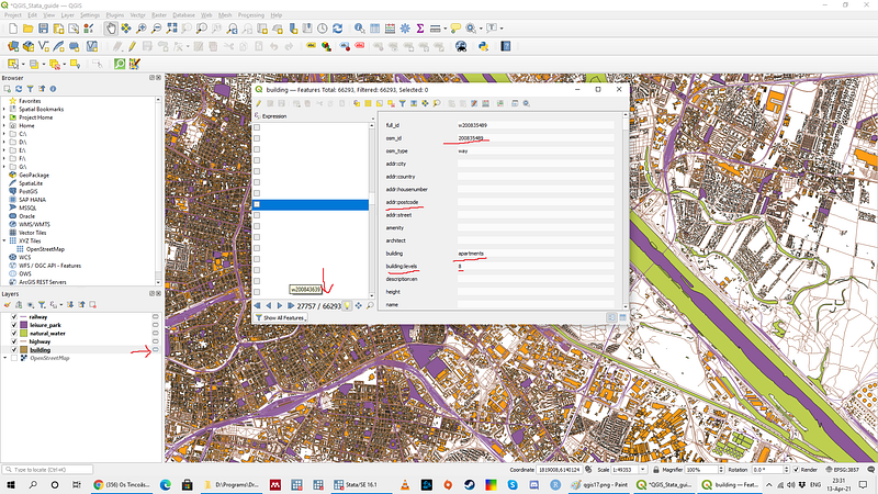
Here we can see that for each building entry, there are dozens of fields most of which are empty. But here we can also find the useful fields for the features we are looking at. For example for buildings there is information on building types, number of floors, postcode etc that can be used for analysis.

Next up, we add the highway layer to get all the roads data. Since roads are basically lines, we get rid of the additional point and polygon data such that we are left with just the road network:

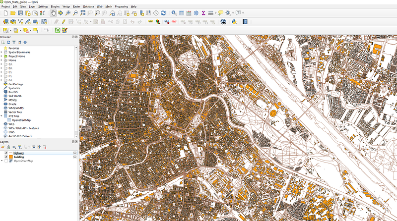
The map is starting to look more like a city. Similar to roads, I I have also added “railways” Key as a map layer (not shown here).

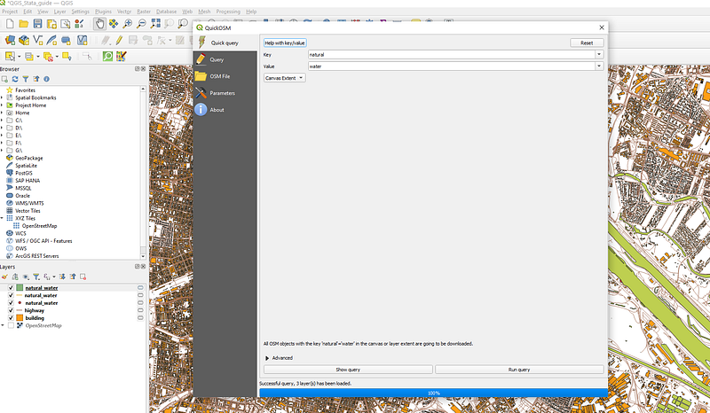
For adding the water, I just select “Natural” key and “water” subkey. I can load more as well but I am just interested in adding the Danube (Donau). Again one can refer to the map features website to find out what we want to add:

Similarly, I just want to add green spaces. These are defined as “leisure” key and “park” value:

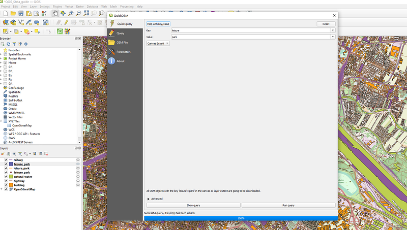
Note that the green spaces are represented as many different names so parks might not cover everything. But for just for the sake of this guide, this is sufficient. For parks we get the following green space:

Here you can see that not all the parks are showing up, especially the Prater park (the main park of Vienna which is three times the size of Central Park in New York) next to the Danube river. You can go on the OSM website and figure out categories by using the identify feature if you want to go for more accuracy:

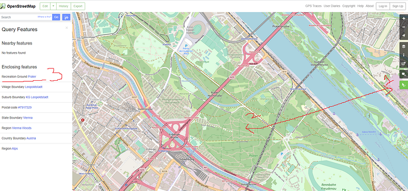
Here we can see that this belongs to the “Recreation ground” category. I can go back and add this feature as well. For this guide, I will just leave it out for now.

Export the layers

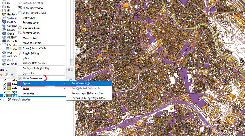
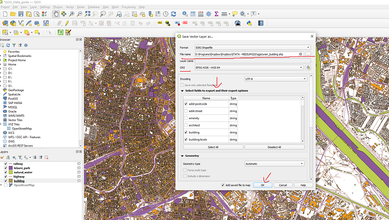
Once all the layers are in order, we can start exporting them to shapefiles that we can read in Stata. To do this, right click on a scratch layer, and click on either Export (or Make Permanent). In the Export menu, click “Save Feature As…”:

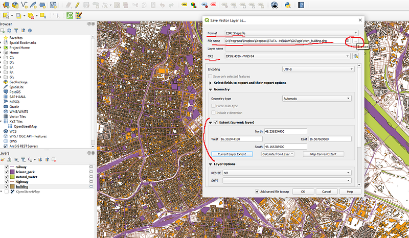
The default format is the ESRI shapefile so we leave it as it is. Next select the directory and the name of the layer. This is the directory which we will also use in Stata. If you are a more advanced user and want to get the right projections, then you can modify the CRS (coordinate reference system) field here. Otherwise best to leave it as the generic WGS 84. The extent should be auto-filled as well:

Since OSM has a lot of fields, some of which have some badly formatted names, the layer will most likely give errors on the export option.

As mentioned earlier, the layer entries can be viewed by right clicking on a layer. Here we press “Deselect All” and just click on the fields we need. For each layer these will be two to three useful fields. Once the fields are selected, click on OK and export the layer:

I won’t show all the layers, but below are some examples of the fields we want to extract:

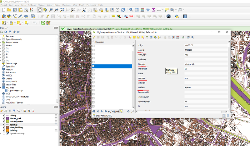
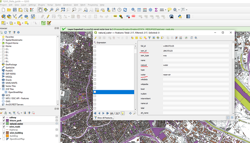
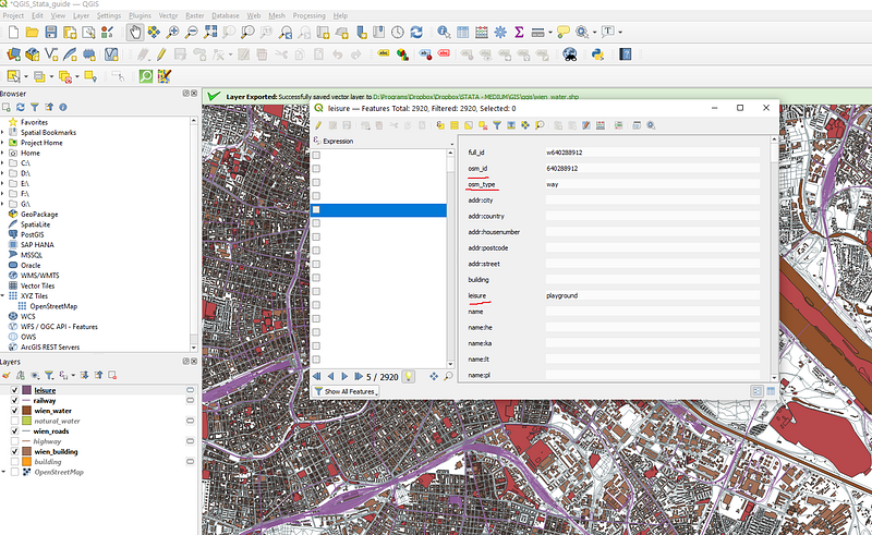
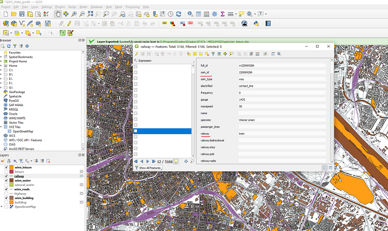
I am showing these since we will process these fields in Stata later. You can either use exactly these ones, or modify the Stata code to fit the layer attributes that you have selected.

Next step, export all the shapefiles in the same folder:

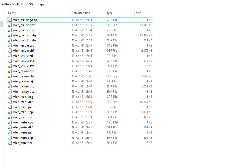
This is the raw data we need to proceed to Stata.

Part II: Stata

Stata 15+ has the ability to read and convert shapefiles to Stata format. This is done as follows:

clear
cd "D:/Programs/Dropbox/Dropbox/STATA - MEDIUM"
cd "GIS/qgis"

********* get the shapefiles in order in order

spshape2dta "wien_building.shp", replace saving(wien_building)
spshape2dta "wien_leisure.shp" , replace saving(wien_leisure)
spshape2dta "wien_roads.shp"   , replace saving(wien_roads)
spshape2dta "wien_water.shp"   , replace saving(wien_water)
spshape2dta "wien_railway.shp" , replace saving(wien_railway)

Keep the names clean and similar to the original files (a good practice to avoid losing track). This is a one time step, so once the layers are converted, mark them out by using the asterisk * before the start of the line *spshape2dta.

Each converted file will create a shape layer file that contains the shape information (_shp.dta) and an attributes layer data file. Since I have covered this extensively in the first two guides here and here, I won’t discuss these in detail here.

Next step, we merge the shape and attribute layers for each layer type:

foreach x in building leisure roads water railway {
 
 use wien_`x'_shp.dta, clear
  merge m:1 _ID using wien_`x'
  gen layer = "`x'"  // for identifying each layer
  order layer
  drop _m
  compress
  save wien_`x'_data.dta, replace
 
}

After this, we stack all these layers together:

****** put the layers together and clean up

use wien_building_data, clear
 append using wien_leisure_data
 append using wien_roads_data
 append using wien_water_data
 append using wien_railway_data

// drop unnecessary variables
drop rec_header
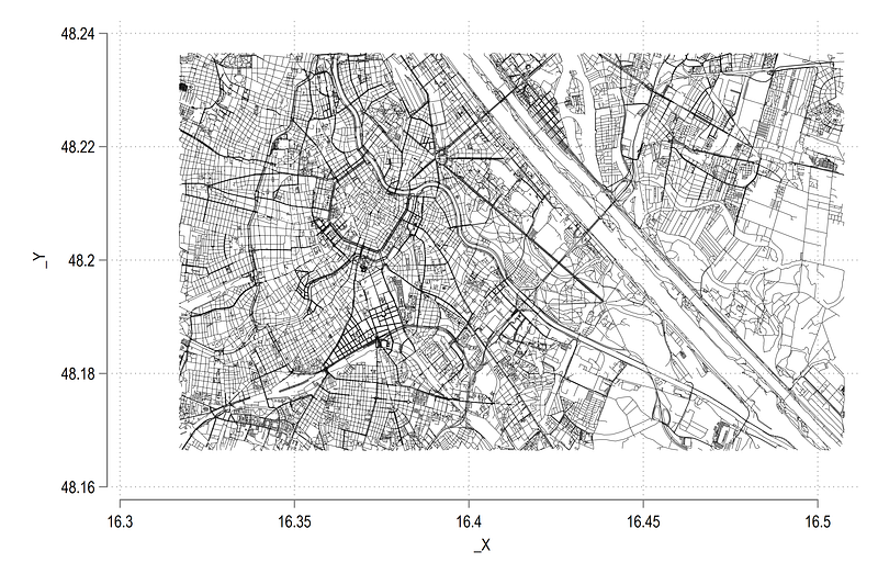
drop osm_id

Since each outline is defined by the {_X, _Y} pair in the data, we can see what the raw map looks like:

twoway (scatter _Y _X,  msymbol(point) msize(small))

For our layers we get this map:

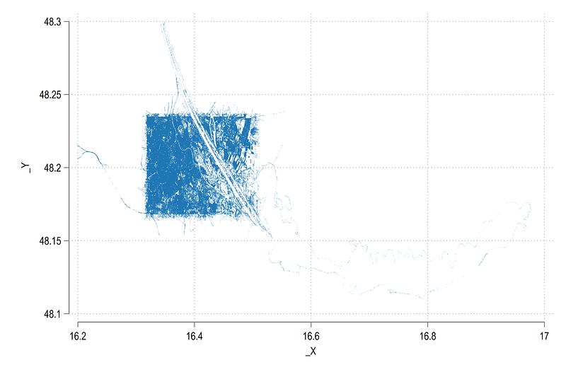
What we see above is that some layers were exported more than the extent of the window. This is not unusual especially if large features like rivers, roads, parks are in the map extent window. If they are, then the whole shape feature will be exported.

In this case, we need to “box” the data to get the map extent that we want. In order to do this, we take a layer that we know has the right extent feature. For example, the building layer:

twoway (scatter _Y _X if layer=="building",  msymbol(point) msize(small))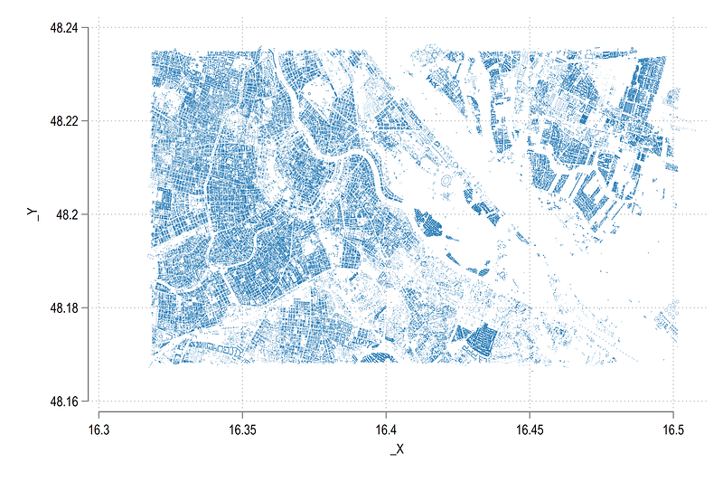

We can use the min/max of this layer and define the box as follows:

summ _X if layer=="building"
gen boxx = 1 if inrange(_X, `r(min)', `r(max)')

summ _Y if layer=="building"
gen boxy = 1 if inrange(_Y, `r(min)', `r(max)') 
 
gen box = 1 if boxx==1 & boxy==1
replace box = 1 if _X==. & _Y==.  //  this is extremely important

keep if box==1

One can define the min/max values independently as well but this is case dependent. Also please keep the empty _X, _Y features in the box==1 variable. This is extremely important to prevent Stata from crashing since the drawing order depends on this.

Here, I would like to highlight that this step also have an advantage over the spmap package. Here we can control what is drawn in the map by limiting the extent of the layers we want to draw. In spmap we either fully include or drop a shape layer.

We can now draw the map again:

twoway (scatter _Y _X,  msymbol(point) msize(small))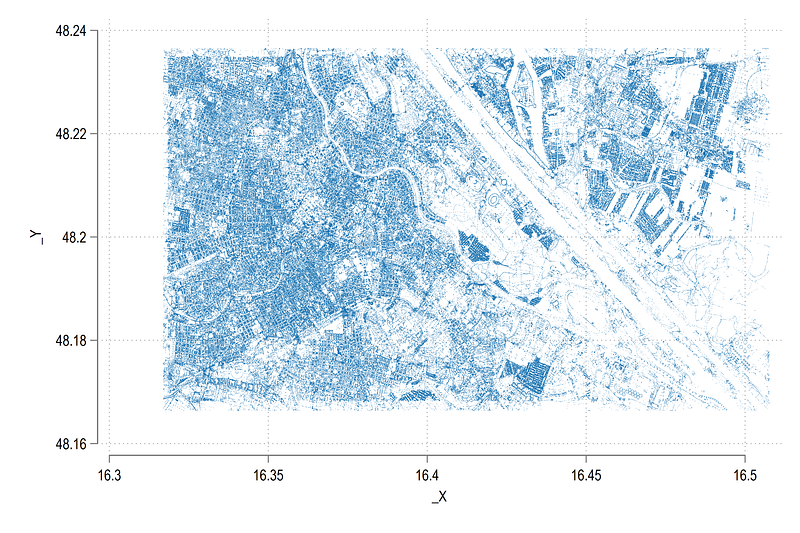

and we get what we want. Note here that I not going in the dimensions or projections of the spatial layers to improve the accuracy of the displayed map. These can be fine tuned and I did discuss these in the second maps guide.

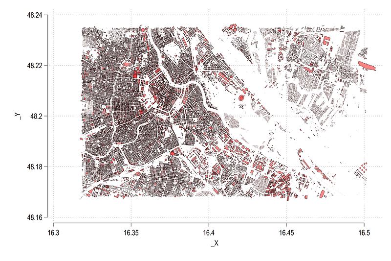
Once the layers are in place, we can draw polygons and color them. For example for buildings:

twoway ///
 (area _Y _X if layer=="building", nodropbase cmissing(n) fc(red%60) lc(black) lw(0.06))  ///   
  , legend(off)

we get:

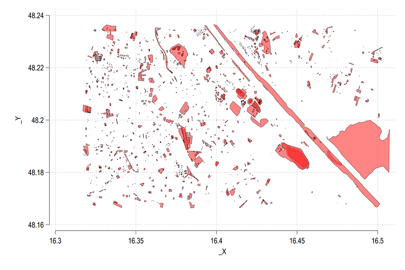
We can draw and check other layers as well:

twoway ///
 (area _Y _X if layer=="leisure", nodropbase cmissing(n) fc(red%60) lc(black) lw(0.06))  ///   
  , legend(off)

twoway ///
 (line _Y _X if layer=="railway", nodropbase cmissing(n) lc(black) lw(0.06))  ///   
  , legend(off)

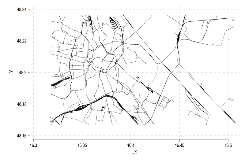
twoway ///
 (line _Y _X if layer=="roads", nodropbase cmissing(n) lc(black) lw(0.06))  ///   
  , legend(off)

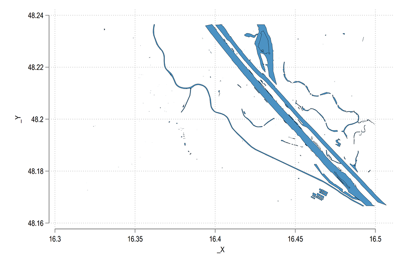
twoway ///
 (area _Y _X if layer=="water", nodropbase cmissing(n) lc(black) lw(0.06))  ///   
  , legend(off)

note we use area and line for different layer types. Point data can also be added simply by using the scatter option. From the above code we get these four layers:

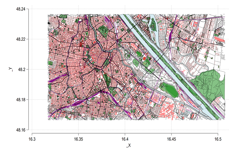
Let’s put them all in one figure:

twoway ///
 (area _Y _X if layer=="water"  , nodropbase cmissing(n) fc(ltblue%60) lc(black) lw(0.06))  ///
 (area _Y _X if layer=="leisure"  , nodropbase cmissing(n) fc(green%60) lc(black) lw(0.06))  /// 
 (area _Y _X if layer=="building" , nodropbase cmissing(n) fc(red%60) lc(black) lw(none))  /// 
 (line _Y _X if layer=="railway"  , nodropbase cmissing(n) lc(purple) lw(0.06))  /// 
 (line _Y _X if layer=="roads"  , nodropbase cmissing(n) lc(black) lw(0.06))  ///
 , legend(off)

Here we get our first baseline map which resembles Vienna:

The axes in the figure above represent latitudes and longitudes. These can be formatted to show map grids but for now, I will drop them:

summ _Y 
local ymin = r(min)
local ymax = r(max)

summ _X 
local xmin = r(min)
local xmax = r(max) 
 
 
twoway ///
 (area _Y _X if layer=="water"  , nodropbase cmissing(n) fc(ltblue%60) lc(black) lw(0.06))  ///
 (area _Y _X if layer=="leisure"  , nodropbase cmissing(n) fc(green%60) lc(black) lw(0.06))  /// 
 (area _Y _X if layer=="building" , nodropbase cmissing(n) fc(red%60) lc(black) lw(none))  /// 
 (line _Y _X if layer=="railway"  , nodropbase cmissing(n) lc(purple) lw(0.06))  /// 
 (line _Y _X if layer=="roads"  , nodropbase cmissing(n) lc(black) lw(0.06))  ///
 , ///
  legend(off) ///
  xtitle("") ytitle("")  ///
   xlabel(`xmin'(0.05)`xmax', nogrid) ylabel(`ymin'(0.05)`ymax', nogrid) ///
   xscale(off) yscale(off)

In the code above, everything is the same as the previous code, except we limit the axes to the exact range min/max range, and we turn off the grid and axes lines:

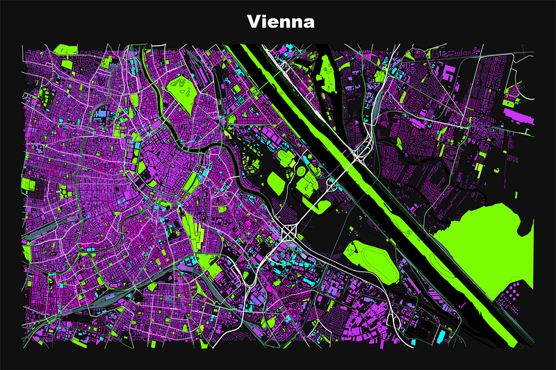
We can also flip the colors the give us a map in negative color space:

summ _Y 
local ymin = r(min)
local ymax = r(max)

summ _X 
local xmin = r(min)
local xmax = r(max) 
 
 
twoway ///
 (area _Y _X if layer=="water"  , nodropbase cmissing(n) fc(ltblue%60) lc(black) lw(0.04))  ///
 (area _Y _X if layer=="leisure"  , nodropbase cmissing(n) fc(green%40) lc(black) lw(0.04))  /// 
 (line _Y _X if layer=="railway"  , nodropbase cmissing(n) lc(yellow%50) lw(0.02))  /// 
 (area _Y _X if layer=="building" , nodropbase cmissing(n) fi(100) fc(pink%60) lc(white) lw(0.02))  /// 
 , ///
  legend(off) ///
  xtitle("") ytitle("")  ///
   xlabel(`xmin'(0.05)`xmax', nogrid) ylabel(`ymin'(0.05)`ymax', nogrid) ///
   xscale(off) yscale(off)  ///
   title("{fontface Arial Black: Vienna}", color(white)) ///
    graphregion(fcolor(black) lcolor(black)) plotregion(fcolor(black) lcolor(black))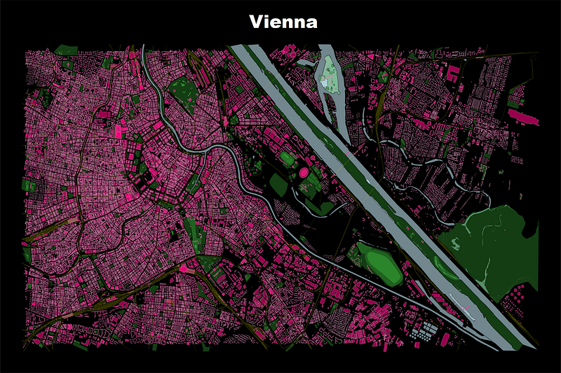

Here one can also start experimenting with various color variations. For example a simple black and white street map also looks nice:

summ _Y 
local ymin = r(min)
local ymax = r(max)

summ _X 
local xmin = r(min)
local xmax = r(max) 
 
 
twoway ///
(line _Y _X if layer=="roads"  , nodropbase cmissing(n) lc(white) lw(0.08))  /// 
 , ///
  legend(off) ///
  xtitle("") ytitle("")  ///
   xlabel(`xmin'(0.05)`xmax', nogrid) ylabel(`ymin'(0.05)`ymax', nogrid) ///
   xscale(off) yscale(off)  ///
   title("{fontface Arial Black: Vienna}", color(white)) ///
    graphregion(fcolor(black) lcolor(black)) plotregion(fcolor(black) lcolor(black))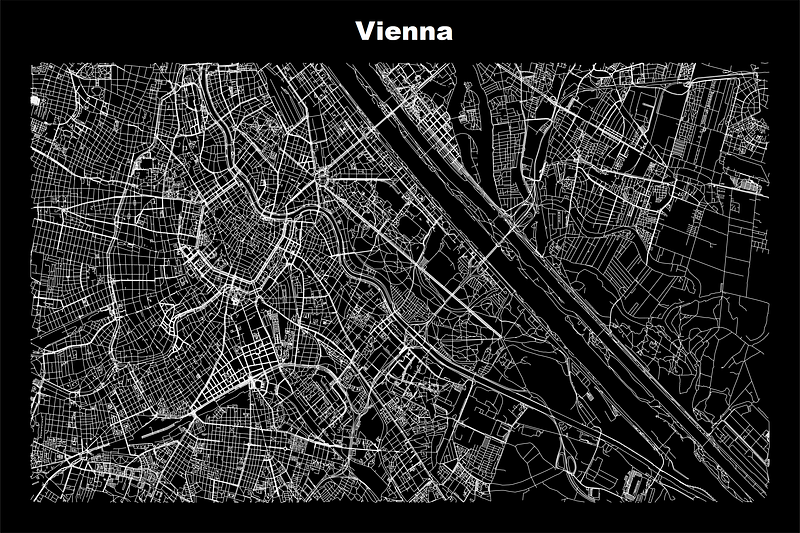

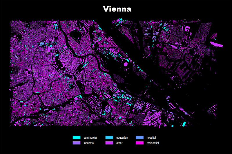
But what if we want to add different color shades to each layer? For example we generate colors by different building types. We can make use of the variables we have exported from OSM and use them to generate some meaningful categories. For example, below I reduce the layers of the building variable:

tab building
replace building = "" if building=="yes"
tab building

cap drop total 
cap drop temp

gen temp = 1 if layer=="building"
bysort building: egen total = total(temp)  if layer=="building"

tab building if total > 0

gen  building_type = building if total > 1000 & layer=="building"
replace building_type="other" if total<= 1000 & layer=="building"

If a building type has more than 1000 features, then this information is retained, otherwise it is assigned to the “other” category. For my specific layer, I cut the categories even more:

replace building_type="commercial" if building_type=="retail"
replace building_type="commercial" if building_type=="office"
replace building_type="commercial" if building_type=="hotel"
replace building_type="residential" if building_type=="house"
replace building_type="residential" if building_type=="apartments"

replace building_type="education" if building_type=="school"
replace building_type="education" if building_type=="university"

replace building_type="other" if building_type =="church"
replace building_type="other" if building_type =="detached"
replace building_type="other" if building_type =="roof"
replace building_type="other" if building_type =="shed"
replace building_type="other" if building_type =="garage"
replace building_type="other" if building_type =="public"
replace building_type="other" if building_type =="greenhouse"
replace building_type="other" if building_type =="train_station"
replace building_type="other" if building_type=="" & layer=="building"

tab building_type

Here feel free to keep, drop, collapse, categories however you want. In the end, my own building_type variable has six categories in total that I want to differentiate by colors.

Next using a combination of locals and loops we auto generate the areas and legend entries and draw the map:

encode building_type, gen(building_type2)

**** draw building type map

sort _ID shape_order

levelsof building_type2, local(lvls)
return list
local shapes = `r(r)'

local i = 1  // counter for colors and legends

foreach x of local lvls {

colorpalette matplotlib cool, n(`shapes') nograph 

 // shape colors
 local buildings `buildings' (area _Y _X  if building_type2==`x', nodropbase cmissing(n) fi(100) fc("`r(p`i')'") lc(gs4)  lw(none)  lp(solid)) ||

// legend entries
 local mylab : label building_type2 `i'
 local legend `legend' lab(`i' "`mylab'")
 
 local i = `i' + 1
}

summ _Y if layer=="building"
local ymin = r(min)
local ymax = r(max)

summ _X if layer=="building"
local xmin = r(min)
local xmax = r(max)

twoway /// 
 `buildings' ///
  , ///
   xlabel(, labsize(vsmall)) ///
   ylabel(, labsize(vsmall)) ///
   legend(`legend' position(6) rows(2) size(vsmall) color(white) region(fcolor(none))) ///
   xtitle("") ytitle("")  ///   
   xlabel(`xmin'(0.05)`xmax', nogrid) ylabel(`ymin'(0.05)`ymax', nogrid) ///
   xscale(off) yscale(off)  ///
   title("{fontface Arial Black: Vienna}", color(white)) ///
    graphregion(fcolor(black) lcolor(black)) plotregion(fcolor(black) lcolor(black))

And we get this layer:

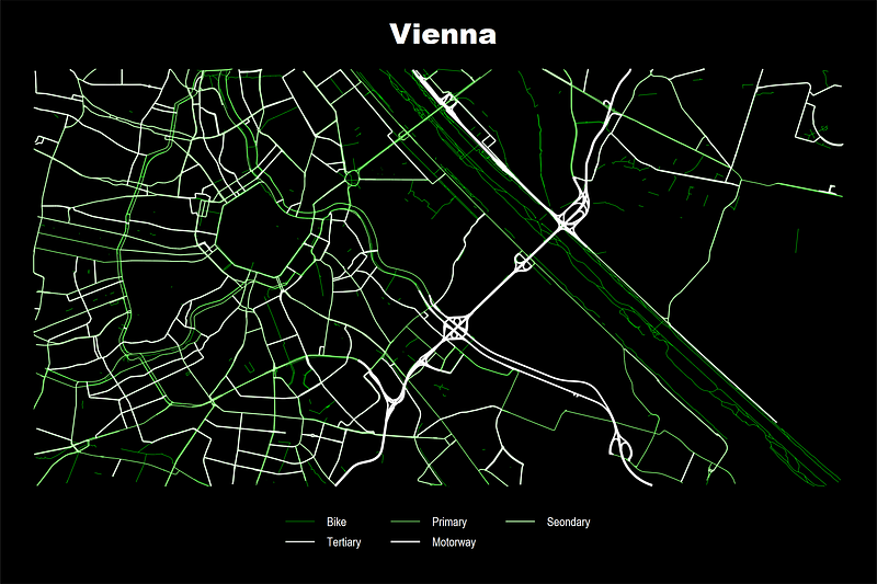
Similarly for roads we can also create a clean variable:

**** Roads and paths

tab highway

gen road = .
replace road = 1 if highway=="cycleway" 
replace road = 2 if highway=="primary" | highway=="primary_link" 
replace road = 3 if highway=="secondary" | highway=="secondary_link"
replace road = 4 if highway=="tertiary"  | highway=="tertiary_link"
replace road = 5 if highway=="motorway"  | highway=="motorway_link"

lab de road 1 "Bike" 2 "Primary" 3 "Secondary" 4 "Tertiary" 5 "Motorway", replace
lab val road road

Depending on the area you are drawing, these categories might vary. I have also dropped all the very minor roads and just taking the broad primary, secondary, and tertiary roads.

We can now draw this layer where we not only modify the color but also the line thickness:

sort _ID shape_order

levelsof road, local(lvls)
return list
local shapes = `r(r)'

local i = 1

foreach x of local lvls {

colorpalette lime white, n(`shapes') nograph
 
 local lw = 0.06 * `i'
 
 local roads `roads' (line _Y _X  if road==`x', nodropbase cmissing(n) lc("`r(p`i')'")  lw(`lw')  lp(solid)) || 
 
 local mylab : label road `i'
 local legend `legend' lab(`i' "`mylab'")
 
 local i = `i' + 1
}   
 
qui summ _Y if layer=="building"
local ymin = r(min)
local ymax = r(max)

qui summ _X if layer=="building"
local xmin = r(min)
local xmax = r(max) 
 
twoway /// 
 `roads' ///
  , ///
   xlabel(, labsize(vsmall)) ///
   ylabel(, labsize(vsmall)) ///
   legend(`legend' position(6) rows(2) color(white)  size(vsmall) region(fcolor(none))) ///
   xtitle("") ytitle("")  ///   
   xlabel(`xmin'(0.05)`xmax', nogrid) ylabel(`ymin'(0.05)`ymax', nogrid) ///
   xscale(off) yscale(off)  ///
   title("{fontface Arial Black: Vienna}", color(white)) ///
    graphregion(fcolor(black) lcolor(black)) plotregion(fcolor(black) lcolor(black))

and we get the broad road network. All the minor arteries are missing. Here we can see the ring around the inner city and the roads along the Danube and the green lines represent exclusive bike paths:

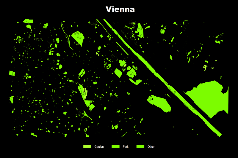
For parks and green spaces:

tab leisure

gen green = .

replace green = 1 if leisure=="garden"
replace green = 2  if leisure=="park"
replace green = 3  if green==. & layer=="leisure"
   
lab de green 1 "Garden" 2 "Park" 3 "Other"   
lab val green green
   
   
levelsof green, local(lvls)
return list
local shapes = `r(r)' + 5

local i = 1

foreach x of local lvls {

colorpalette HTML green, n(`shapes') nograph
 
 local green `green' (area _Y _X  if green==`x', nodropbase cmissing(n) fi(100) fc("`r(p`i')'") lc(black)  lw(0.04)  lp(solid)) || 
 
 local mylab : label green `i'
 local legend `legend' lab(`i' "`mylab'")
 
 local i = `i' + 1
}

summ _Y if layer=="building"
local ymin = r(min)
local ymax = r(max)

summ _X if layer=="building"
local xmin = r(min)
local xmax = r(max)

twoway /// 
 `green' ///
  , ///
   xlabel(, labsize(vsmall)) ///
   ylabel(, labsize(vsmall)) ///
   legend(`legend' position(6) rows(1) color(white)  size(vsmall) region(fcolor(none))) ///
   xtitle("") ytitle("")  ///   
   xlabel(`xmin'(0.05)`xmax', nogrid) ylabel(`ymin'(0.05)`ymax', nogrid) ///
   xscale(off) yscale(off)  ///
   title("{fontface Arial Black: Vienna}", color(white)) ///
    graphregion(fcolor(black) lcolor(black)) plotregion(fcolor(black) lcolor(black))

Here color differentiation is very minor. This can be fine tuned as well but I leave it as it is for now. Here we can see the Donauinsel (Danube Island) running in the middle of the Danube river:

For railways we can differentiate by rail types:

**** Railways

tab railway

gen rail = .
replace rail = 1 if railway=="rail"
replace rail = 2 if railway=="tram" | railway=="tram_stop"
replace rail = 3 if railway=="subway"
replace rail = 4 if railway=="other"

lab de rail 1 "Rail" 2 "Tram" 3 "Subway" 4 "Other"
lab val rail rail

sort _ID shape_order

levelsof rail, local(lvls)
local shapes = `r(r)'

local i = 1

foreach x of local lvls {

colorpalette HTML blue, n(`shapes') nograph
 
 
local rails `rails' (line _Y _X  if rail==`x', nodropbase cmissing(n) lc("`r(p`i')'")  lw(0.05)  lp(solid)) || 
 
 local mylab : label rail `i'
 local legend `legend' lab(`i' "`mylab'")
 
 local i = `i' + 1
}   
 
summ _Y if layer=="building"
local ymin = r(min)
local ymax = r(max)

summ _X if layer=="building"
local xmin = r(min)
local xmax = r(max) 
 
twoway /// 
 `rails' ///
  , ///
   xlabel(, labsize(vsmall)) ///
   ylabel(, labsize(vsmall)) ///
   legend(`legend' position(6) rows(1) color(white)  size(vsmall) region(fcolor(none))) ///
   xtitle("") ytitle("")  ///   
   xlabel(`xmin'(0.05)`xmax', nogrid) ylabel(`ymin'(0.05)`ymax', nogrid) ///
   xscale(off) yscale(off)  ///
   title("{fontface Arial Black: Vienna}", color(white)) ///
    graphregion(fcolor(black) lcolor(black)) plotregion(fcolor(black) lcolor(black))

And we get the public transport infrastructure:

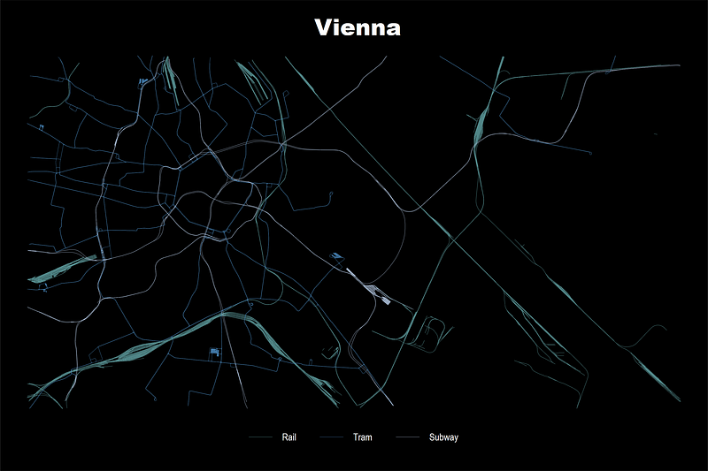
The main train station (Haupbahnhof) is visible in the bottom left of the map together with the various tracks that emerge from it.

Next step, let’s put all these layers together!

sort _ID shape_order

local roads
local rails
local buildings
local leisure

// roads
levelsof road, local(lvls)
local shapes = `r(r)'

local i = 1
foreach x of local lvls {
 colorpalette lime white, n(`shapes') nograph
 
 local lw = 0.03 * `i' 
 local roads `roads' (line _Y _X  if road==`x', nodropbase cmissing(n) lc("`r(p`i')'")  lw(`lw')  lp(solid)) || 
 
 local mylab : label road `i'
 local legend `legend' lab(`i' "`mylab'") 
  local i = `i' + 1
}

// rails

levelsof rail, local(lvls)
local shapes = `r(r)'

local i = 1
foreach x of local lvls {
 colorpalette HTML blue, n(`shapes') nograph
 
 local rails `rails' (line _Y _X  if rail==`x', nodropbase cmissing(n) lc("`r(p`i')'")  lw(0.04)  lp(solid)) || 
 
 local mylab : label rail `i'
 local legend `legend' lab(`i' "`mylab'")
  local i = `i' + 1
}

// Leisure

levelsof green, local(lvls)
local shapes = `r(r)' + 5

local i = 1

foreach x of local lvls {
 colorpalette HTML green, n(`shapes') nograph
 
 local green `green' (area _Y _X  if green==`x', nodropbase cmissing(n) fi(100) fc("`r(p`i')'%50") lc(black)  lw(0.04)  lp(solid)) || 
 local mylab : label green `i'
 local legend `legend' lab(`i' "`mylab'")
  local i = `i' + 1
}

// building

levelsof building_type2, local(lvls)
local shapes = `r(r)'

local i = 1

foreach x of local lvls {

colorpalette matplotlib cool, n(`shapes') nograph 
 
 local buildings `buildings' (area _Y _X  if building_type2==`x', nodropbase cmissing(n) fi(100) fc("`r(p`i')'") lc(gs4)  lw(none)  lp(solid)) || 
 local mylab : label building_type2 `i'
 local legend `legend' lab(`i' "`mylab'")
  local i = `i' + 1
}

// get the axes extents

summ _Y if layer=="building"
local ymin = r(min)
local ymax = r(max)

summ _X if layer=="building"
local xmin = r(min)
local xmax = r(max)

// plot the data 
 
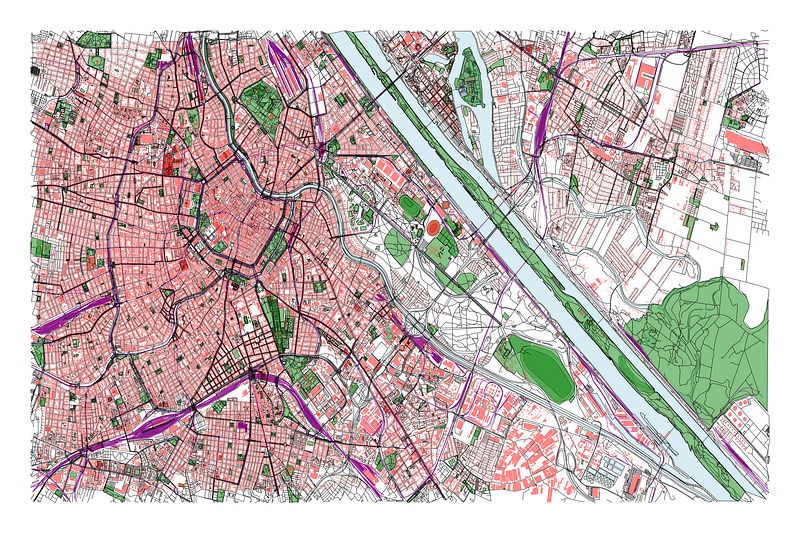
twoway /// 
 (area _Y _X if layer=="water"  , nodropbase cmissing(n) fi(100) fc(black) lc(black) lw(none))  ///
 `buildings' ///
 `green' ///
 `rails' ///
 `roads' ///
  , ///
   xlabel(, labsize(vsmall)) ///
   ylabel(, labsize(vsmall)) ///
   legend(off) ///
   xtitle("") ytitle("")  ///   
   xlabel(`xmin'(0.05)`xmax', nogrid) ylabel(`ymin'(0.05)`ymax', nogrid) ///
   xscale(off) yscale(off)  ///
   title("{fontface Arial Black: Vienna}", color(white)) ///
    graphregion(fcolor(gs1) lcolor(gs1)) plotregion(fcolor(gs1) lcolor(gs1))

The steps above are the same as defined earlier. Here I have done some very minor tweaks to colors and lines. The background is not fully black (it usually never is on websites with a dark background). From the code above, we get the map of the city of Vienna:

These colors can be modified and customized according to taste. Personally, I am exploring inverted color schemes just to get away from the white background, and I like the version above that I came up with. The city map can be refined further (for example Prater park is missing) but here you get the idea of how to working with spatial layers and colors in Stata.

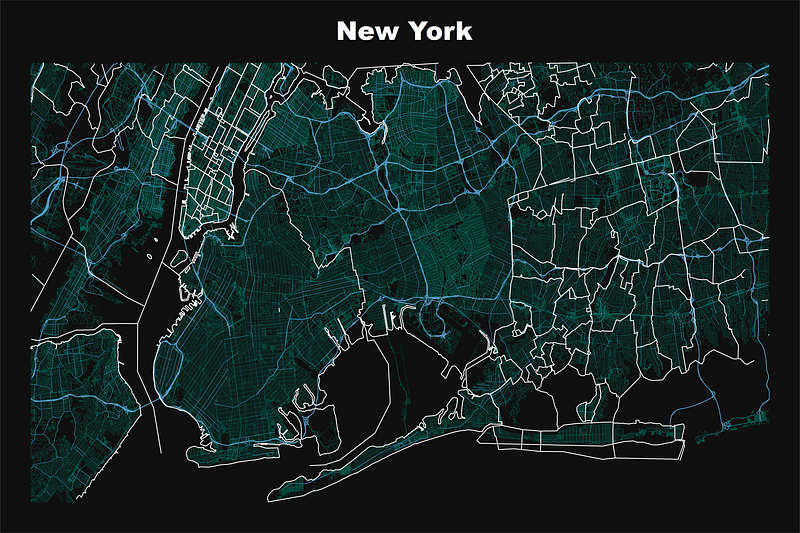
Below you can see a map of New York, focusing on Brooklyn (since I lived there :). Here I am using the road layer network with colors and line widths differentiated by road type. In addition to this, I have added the “administrative” boundary key layer as well. It contains more data than I need but it delineated the state of New York from New Jersey and highlights the Islands as well.

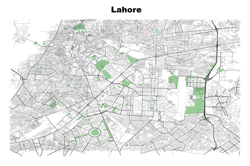
Last map, is my home town of Lahore featured in a white background map. Lahore is a city of 12 million people on the east side of Pakistan along the border with India. It has endless amounts of roads. The circular Model Town park and cross are visible on the map (bottom left) and also the airport (center right) and the walled inner city (top left).

If I make more city maps, I will add them here in the future. Hope you enjoyed this guide! Please share your maps as well including other color schemes you have used.

About the author

I am an economist by profession and I have been using Stata since 2003. I am currently based in Vienna, Austria where I work at the Vienna University of Economics and Business (WU) and at the International Institute for Applied Systems Analysis (IIASA). You can find my research work on ResearchGate and Google Scholar, and Stata code repository on GitHub. You can follow my COVID-19 related Stata visualizations on Twitter. I am also featured on the Stata COVID-19 webpage in the visualization and graphics section.

You can connect with me via Medium, Twitter, LinkedIn or simply via email: [email protected].

The Stata Guide, releases awesome new content regularly. Clap, and/or follow if you like these guides!