Identify Causality by Regression Discontinuity

In data analytic projects we are asked to deliver “business sense” as well as accuracy in “model prediction”. What is business sense? It means the insights that stakeholders can take action. It is about the causality between the dependent and explanatory variables. In the article “Machine Learning or Econometrics”, I elaborated that machine learning techniques are good at precision and efficiency, while econometric techniques are good at identifying causality. A machine learning model can render accuracy in prediction, however, it is not designed to identify causality. I have written a list of articles on machine learning techniques. You can bookmark “Dataman Learning Paths — Build Your Skills, Drive Your Career” to find more.

In the “identify causality” series of articles, I present econometric techniques that identify causality. These articles cover the following techniques:

• Machine Learning or Econometrics? (see “Machine Learning or Economics?”
• Regression Discontinuity (see “Identify Causality by Regression Discontinuity”),
• Difference in differences (DiD)(see “Identify Causality by Difference in Differences”),
• Fixed-Effects Models (See “Identify Causality by Fixed-Effects Models”),
• Randomized Controlled Trial with Factorial Design (see “Design of Experiments for Your Change Management”).

In each article, I present the applications in various fields so you see the formation of their problems. I then offer the best practices, the sample code, and how to conclude.

Randomized Controlled Trials (RCT) may not be feasible

An RCT seems to be the most intuitive scientific method to test the impact of an intervention. You randomly put some subjects into the treatment group and control group to compare the results of the two groups. However, RCTs can be time-consuming, expensive, and hard to explain to the public yet whose cooperation is needed, and the selection criteria can sometimes be viewed as unethical. For example, in a hospital setting a researcher may suggest withholding patients be the control group. This may not be feasible because the research puts the patient's health condition at risk. Not all policy questions or clinical experiments can follow RCT. What else can we do? Researchers have increasingly relied on quasi-experimental designs and achieved compelling results.

What Is a Quasi-experimental Design?

The word quasi means seemingly, apparently but not really. A quasi-experiment design is similar to a randomized controlled trial but without the random assignments by the researcher (Cook & Campbell, 1979). Although researchers do not have the freedom to randomly assign subjects into test and control groups, the subjects being tested are largely random. Researchers can use some criterion (such as a threshold) for selection and the results can be proven. In a quasi-experiment, the only difference between the treatment group and the control group is the treatment itself. In such a design, we can say the process is “as good as random”. The Regression Discontinuity (RD) design in this article is a type of quasi-experimental approach.

What Is Regression Discontinuity (RD)?

The RD design compares subjects that are just above and just below the threshold, as shown in the green box in the “Before” scenario of Figure (A). The subjects in the green box are expected to be very similar. In the “After” scenario the right group receives an intervention and has a different result. This jump or discontinuity in outcomes can be interpreted as the consequence of the intervention.

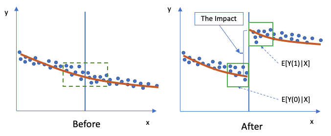
The expected impact on Y in the “after” period (“1”=after) is E[Y(1)|X] and the “before” period (“0”=before) is E[Y(0)|X]. All the Xs are very similar in the small green box, so the Xs in the “before” and “after” periods are considered the same.

Regression Discontinuity Applications in Clinical Studies

The RD designs have been widely used in health policy, public health, and clinical services. Clinical threshold rules based on continuously measured biomarkers (such as CD4) are common applications of regression discontinuity. Bor et al (2014) show that in Africa people with a CD4 count just below the 200 cells/mm threshold had a 35% lower hazard of death than those with CD4 counts just above it. They proved patients just above and just below the threshold were statistically identical across baseline characteristics. For readers who may not come from a medical background, CD4 cells are white blood cells that fight infection, and the CD4 count measures how well your immune system is. As HIV infection progresses, the number of these cells declines. When the CD4 count drops below 200, a person is diagnosed with AIDS. A normal range for CD4 cells is about 500–1,500.

Regression Discontinuity Applications in Education Policies

The RD design is also used in assessing academic outcomes regarding a particular policy. For example, do the maximum class-size rules affect academic outcomes? One can compare classes just above and just below the class-size threshold (Leuven et al 2008). Another example is the school-entry cut-off dates. Do school-entry cut-off dates affect academic outcomes? Children born just before or after the cut-off dates become two different academic grades and are expected to perform differently (Bedard and Dhuey 2006; Puhani & Weber 2007).

Regression Discontinuity Applications in Public Policies

“Does alcohol consumption by young adults increase mortality?” Understanding whether there is a causal link between youth alcohol consumption and mortality has direct public policy implications. This seemingly easy question is not easy because it requires the consideration of heterogeneous factors. There are many causes of death among young adults such as suicide, drug overdose, alcohol overdose, homicide, or even the high-way speed limit in a state. How can we conclude the minimum legal drinking age (MLDA) causes mortality?

In the paper “The Effect of Alcohol Consumption on Mortality: Regression Discontinuity Evidence from the Minimum Drinking Age” by Christopher Carpenter and Carlos Dobkin (2009), the authors successfully identified the causality and measured the impact using regression discontinuity. The RD process is summarized in the following:

• The MLDA presents sharp differences in alcohol access for young adults on either side of age 21.
• The observed and unobserved determinants of alcohol consumption and mortality are likely to trend smoothly across the age-21 threshold.
• The jumps in mortality at age 21 and alcohol consumption indicate the causal effect of alcohol consumption on mortality among young adults.
• The RD empirical results provide compelling graphical and regression-based evidence that the MLDA laws result in sharp differences in alcohol consumption and mortality for youths on either side of the age-21 threshold.

Data Analysis

The dataset of the above MLDA research is available here. The origin dataset is in Stata. I am going to use Python to conduct the analysis.

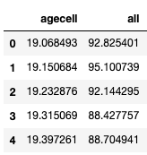
There are 48 observations after dropping two records with a missing value. The variables of interest are the drinking age and the total count of deaths, i.e, “agecell” and “all”.

(A) Binning is an Important Step

The age variable is binned into 10 equal groups. Then we use box-plotting to present the count of deaths against the binned age group. (If you are not sure how to use Seaborn for data visualization, you can check “Use Seaborn to Do Beautiful Plots Easy!”)

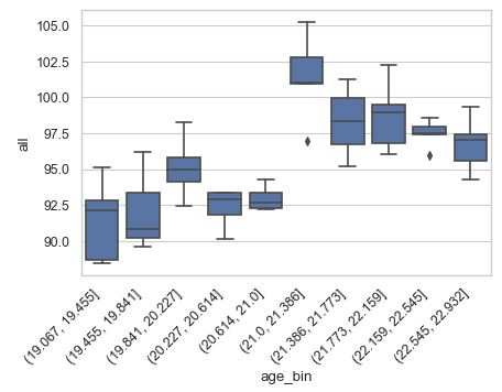
Choosing the right “bin width” is an important task in visualizing discontinuity. Without binning the rating variable, the plot will be too noisy to see. On the other hand, if there are only four bins or fewer, the discontinuity may be hard to find. You can test a range of equal groups. In our case, the 10 equal groups seem appropriate.

(B) Observations Around the Threshold Are Random

An intuitive assumption in the RD analysis is that differences between observations that are just below or just above the threshold are random. In our case, the MLDA is 21 years old. What about a young adult who is 20.9 years old and another one is 21.1 years old? Because the policy is applied to those ≥21 years old, any difference in subsequent mean outcomes must, therefore, be caused by the policy.

(C) Functional Form

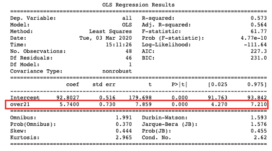
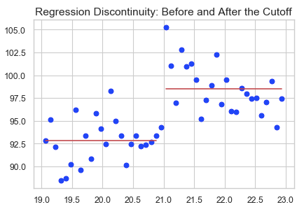
The simplest form is a linear regression: Y_i = a + b * T_i, where Y_i is the outcome measure for observation i, T_i = 1 if observation i is in the treatment group and 0 otherwise. In our case the dichotomous variable “over21” is T_i. We perform a simple ordinary least square (OLS) regression. The results show that coefficient b is statistically significant at 95%, meaning the jump in the outcome is statistically significant. In other words, the MLDA increases mortality (as shown in the graph).

(D) Some Assumptions about The Rating Variable

• The rating variable (“age” in our case) cannot be endogenous — caused by or influenced by the treatment.
• The selection for the cut-point (“21” in our case) should be exogenous — independent of the rating variable.

(E) Prove that the Observations around the Threshold Are almost Identical

As mentioned in (B), the differences between observations that are just below or just above the threshold are assumed random. So you need to show the distributions of other factors for observations around the threshold are the same. For example, the gender distribution just above or below the threshold is approximately the same.

(F) Sharp and Fuzzy Design

What if some of the below-21-year-old young adults drink alcohol? The econometric literature further considers two distinct types of RD designs: the sharp design and the fuzzy design. If all subjects receive their assigned treatment or control condition, it is called the sharp design. Our analysis above is the sharp design in which the MLDA law is strictly enforced. If some subjects do not receive, it is called the fuzzy design. This paper provides a good summary of the statistical treatment.