Identify Causality by Fixed Effects Models

It is well known that “correlation does not mean causation”. I am going to tell you, that correlation can mean causation but only when certain conditions hold. These conditions have been discussed extensively in the econometric literature. In this article, I will summarize them in an approachable way. I will explain why the standard Ordinary Least Square (OLS) cannot identify causality if these conditions do not meet. I then introduce the Fixed-Effects (FE) models that can provide an effective solution. After that, I will use two data analysis examples to show you how to do it in python. I hope this article will enhance your causality statement with a robust design and convincing results.

I have written a series of articles on “identify causality” that cover the following econometric techniques:

• Machine Learning or Econometrics? (see “Machine Learning or Economics?”
• Regression Discontinuity (see “Identify Causality by Regression Discontinuity”),
• Difference in differences (DiD)(see “Identify Causality by Difference in Differences”),
• Fixed-Effects Models (See “Identify Causality by Fixed-Effects Models”),
• Randomized Controlled Trial with Factorial Design (see “Design of Experiments for Your Change Management”).

In each article, I present the applications in various fields so you see the formation of their problems. I offer the best practices, the sample code, and how to conclude. You can also bookmark “Dataman Learning Paths — Build Your Skills, Drive Your Career” to find more.

Correlation Can Mean Causation — Only When Certain Conditions Meet

Let’s Give the formal definition of causation. Causation means x results in y. Correlation means x and y move together in the same or opposite direction. Causation should meet the following three classic conditions:

• x must happen before y,
• x must be reliably correlated with y,
• the relation between x and y must not be explained by other causes.

Inferring Causation from Correlation Is a Scary Thing

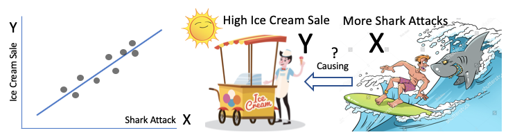
In Figure (A), the increase in ice cream sales correlates strongly with shark attacks in summer. Do you think this makes sense? This is a correlation but not causation because not all of the above three conditions hold. First, the shark attacks do not proceed in an increase in the ice cream sale. Second, the correlation between the increase in ice cream sales and shark attacks may or may not be always true. Third, and most importantly, the relation between the two factors can be explained by the summer season. The summer heat is the driving force that results in increases in ice cream sales and shark attacks.

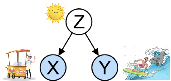
Confounding Factor: Both the ice cream sale x and the shark attacks y are driven by the summer heat, the confounding factor z, as shown in Figure (B). A confounder is a variable that influences both the dependent variable y and the independent variable x, causing a spurious association. The confounding factor may have been omitted in a study. Because we did not collect the data, it is unobservable. The remedy is to identify it as an observable factor.

Endogeneity: If there exists a confounding factor that can explain the relationship between x and y, then x is endogenous. Even the correlation between x and y is not interpretable or is meaningless. Can you claim there is a positive relationship between the ice cream sale and the shark attacks? We should not be tempted to draw any conclusions from the positive or negative signs. The truth is the coefficient can be higher, lower, or even of a different sign.

How to Measure the Effects of X on Y?

To measure the effects of the treatment, we must compare with the counterfactual that there is no treatment. In other words, we ask what the result would be if the individuals did not receive the treatment.

Randomized Control Trial (RCT) is Typically the Gold Standard

How can we ask this difficult question? A Randomized Control Trial (RCT) is typically viewed as the gold standard design because causality is assured (Shadish et al., 2002). If we can randomly assign individuals to treatment and control groups, the characteristics of the individuals will be approximately equal between the two groups. Then the treatment effect is simply the difference in y between the two groups.

If we can randomly assign individuals to treatment and control groups, the characteristics of the individuals will be approximately equal between the two groups. Then the treatment effect is simply the difference in y between the two groups.

Let me use a statistical way to deliver the above description. An Ordinary Least Square (OLS) assumes there is no correlation between x and the unobservable term 𝜺, i.e., there is no endogeneity as described above. This can be achieved in an RCT because the random assignment makes endogeneity or confounding issues very unlikely. An OLS is described in the following equation, where i is the identifier for each of the N individuals. The second equation is in a matrix form. The key assumption is E(X𝜺)=0, which says no correlation between x and the unobservable term 𝜺. The error term can include any unobservable terms.

However, conducting RCTs may not be feasible in most cases. RCTs can be time-consuming, expensive, and hard to explain to the public yet whose cooperation is needed, and the selection criteria can sometimes be viewed as unethical. For example, in a hospital setting a researcher may suggest withholding patients be the control group. This may not be feasible because the research puts the patient's health condition at risk. Not all policy questions or clinical experiments can follow RCT. What else can we do? Researchers have increasingly relied on quasi-experimental designs and achieved compelling results. The word quasi means seemingly, apparently but not really. A quasi-experiment design is similar to a randomized controlled trial but without the random assignments by the researcher (Cook & Campbell, 1979).

Quasi-experiment — Close to Being “As Good As Random”

A lot of studies cannot be done in RCTs. So we use a Quasi-experimental design, in which the only difference between exposed and unexposed units is the exposure itself. The typical quasi-experiments include Regression Discontinuity (RD), Difference-in-differences(DiD), and Fixed-Effects Model (FE).

Regression Discontinuity (RD)

The RD design compares subjects that are just above and just below the threshold, as shown in the green box in the “Before” scenario of Figure (A). The subjects in the green box are expected to be very similar. In the “After” scenario the right group receives an intervention and has a different result. This jump or discontinuity in outcomes can be interpreted as the consequence of the intervention.

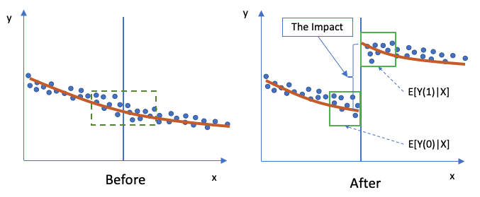
The expected impact on Y in the “after” period (“1”=after) is E[Y(1)|X] and the “before” period (“0”=before) is E[Y(0)|X]. All the Xs are very similar in the small green box, so the Xs in the “before” and “after” periods are considered the same. The results of RD are close to an RCT. In the post “Identify Causality by Regression Discontinuity” I provide a full description of RD.

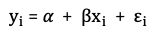
Panel Data: is also called longitudinal or cross-sectional time-series data. In panel data, you have the data points of an individual for all periods. A basic panel data regression model looks like Equation (1), where 𝜶 and 𝜷 are coefficients, and i and t are indices for individuals and time. Panel data allows you to control for variables and account for individual heterogeneity. Interestingly, if you use the Pandas module in Python, you may wonder why the developers call it “Pandas” — cute! It is from “panel data”.

If We Could Specify All Factors Exhaustively and Explicitly in an OLS: Suppose we want to know if a person’s marital status drives a person’s income. Suppose we can specify an exhaustive model that all factors influencing the income level are listed explicitly:

where y_it is the income of person i in time t, x_it is marital status, Z_it are all observed time-varying covariates such as age or number of jobs. W_i are all observed time-invariant covariates like race or ethnicity, and 𝛆_it is the error term. If we can list all the factors, we can get an unbiased estimate for 𝜷.

When you run an OLS on Panel data, it is also called the Pooled OLS. This is appropriate when each observation is independent of any other. The within-panel independence may be unlikely because the observations of the same individual in panel data are related. That being said, sometimes the within-panel correlation of observations is negligibly small. Then you can do so.

But We Are Not Likely to Specify Every Possible Factor in an OLS: Likely, we cannot list all the factors exhaustively in an OLS. Suppose we omit the Z_it and W_i from the above equation and regress only y_it on x_it. We know it is very likely that marital status (x_it), age (Z_it), and ethnicity (W_i) are correlated. Without specifying Z_it and W_i explicitly, the estimate for 𝜷 in an OLS is almost certainly biased. This is because Z_it and W_i are not specified in the equation so they become unobserved and merged to the error term 𝛆_it. This makes the marital status (x_it) endogenous (see the above explanation). So the result 𝜷, either positive or negative, will mean nothing at all. So the issue of omitted variables is very serious. Do not accept the results in an OLS if any known variables are omitted.

Fixed-Effects Models

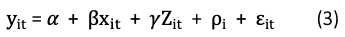
The above 𝝆_i variable is called the fixed effects because it doesn’t change over time. It captures all time-invariant factors of an individual i such as gender, ethnicity, or even personal traits. y_it and x_it are the income and marital status of individual i, and Z_it represents all other time-varying factors of i. The error 𝛆_it is assumed uncorrelated with all terms (if this assumption is violated, we face omitted variables bias.)

How to estimate Equation (3)? In almost all textbooks you see the standard representation like Equation (3). It can be considered as i = 0, 1. When there are multiple individuals i = 1,…N, 𝝆_i can be considered as the shorthand for a set of (N-1) dummy variables D_i with respective coefficient 𝜽_i, as shown in Equation (4), which is what you see in the regression output.

Difference-in-Differences Is a Special Case of the Fixed-Effects Model

Difference-in-Differences (DiD) is a special case of the FE models. In the post “Identify Causality by Difference in Differences” I briefed how DiD can help to identify causal relationships.

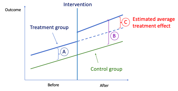
The idea behind DiD is simple. First, we compute the difference in the mean of the outcome between the two groups in the “Before” period, which is “A” in Figure (E). Second, we compute the same for the “After” period, which is “B”. Then we take the “second difference”, which is the difference between (A) and “B” and is labeled as “C”. This second difference measures how the change in outcome differs between the two groups. The difference is attributed to the causal effect of the intervention.

In a panel data form, DiD can be derived from FE models by “differencing out” the confounding factors. Because there is no confounding factor, the effects are indeed causal. The typical setting is like Equation (5).

Suppose individual i is either in the treatment group (x_i = 1) or the control group (x_i = 0), and the pre-period (t_i=1) or the post-period (t_i=0). The effects in the post-period are 𝜷_2, as shown in Figure (E). This is derived by:

The distinction between the DiD models and the FE models is the change is an exogenous shock. The change is made outside of the choice of the individual i. For example, a state changes its minimum drinking age law. This policy is exogenous.

Fixed Effects Data Analysis Example 1 — Investment vs. Market Value

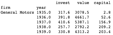
What is the principal driver of the investment of a firm? There is a large literature debating the driving factors. Grunfeld argued that the market value of the firm is the principal explainer and predictor of investment. In the following exercise, I am going to use the Grunfeld dataset (available in statsmodels. datasets) to demonstrate the use of the Fixed-Effects Model. By the way, the Grunfeld Dataset is a well-known dataset in Econometrics, like the iris dataset in Machine Learning. This academic article “The Grunfeld Data at 50” notes its wide usage.

The data has 20 years of data for each of the 11 firms: IBM, General Electric, US Steel, Atlantic Refining, Diamond Match, Westinghouse, General Motors, Goodyear, Chrysler, Union Oil, and American Steel. In the panel data, the “firm” and “year” are set as indices. The fixed-effects model is specified as below, where the individual firm factor is 𝝆_i or called entity_effects in the following code. The time factor is 𝝋_t or called time_effects.

Or as the following, where D_j is the dummy variable for Firm i and I_t is the dummy variable for year t.

The module linearmodels provide PandelOLS to do the fixed-effects models. Turnentity_effects=True to model the firm-specific factor. It means creating 10 (N-1) dummy variables for the 11 firms. Below I show there are two ways to code the regression. Both yield identical results.

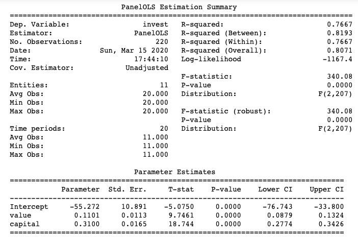
The coefficient of “value” is 0.1101 statistically significant at 95%. Grunfeld, therefore, concluded the causal relationship that high investment is driven by high market value.

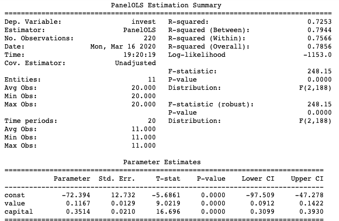
The code below specifies both the firm-specific effects and time effects. And the conclusion stays the same.

Fixed-Effects Data Analysis Example 2 — Traffic Fatality Rate vs. Beer Tax

Does higher beer tax help to reduce the traffic fatality rate? Many states had lowered the beer tax and experienced higher traffic fatality rates. Can we say the decrease in the beer taxes results in higher fatality rates? Such causal effects have profound policy implications. I will use the fatalities dataset in Stock & Watson’s well-recognized book “Introduction to Econometrics”.

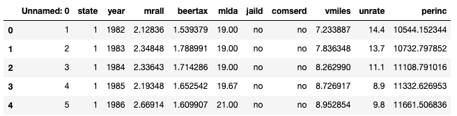
• mrall = total vehicle fatality rate
• beertax = alcohol tax
• mlda = minimum legal drinking age
• jaild = mandatory jail sentence
• comserd = mandatory community service
• vmiles = average mile per driver
• unrate = unemployment rate
• perinc = per capita personal income

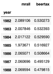
I generate the averages per year to show the average beer tax and fatality rate by year. The average beer taxes in 1982–1984 are higher than those in 1986–1988.

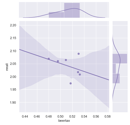
I am going to use seaborn to show the correlation. If you are not familiar with seaborn, you can click “Use Seaborn to Do Beautiful Plot Easy”. The plot shows there is a negative correlation between the fatality rate and the beer tax.

Can we establish any causal relationship? I will use the fixed-effects models to test. Below I demonstrate two fixed-effects models and the pooled OLS for discussion.

• Model 1: Entity_effects + Time_effects
• Model 2: Entity_effects
• Model 3: Pooled OLS

Or as the following, where D_j is the dummy variable for State i and I_t is the dummy variable for year t.

The entity effects control for state time-invariant variables such as state culture, the attitude of the state residents towards drinking (it could be time-invariant), etc. The time effects control for omitted variables that vary over time for all states. For example, the macroeconomic conditions or federal policy measures are common to all states but vary over time.

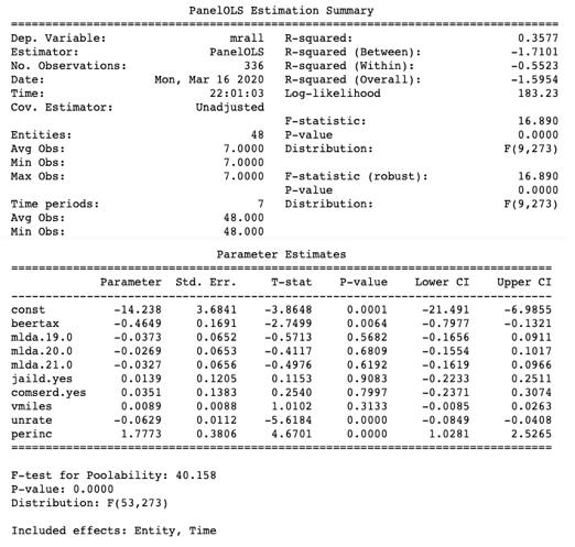
You may ask how to confirm the fixed-effects model specification is needed. It is done by the Poolability Test. Many modules already include the test result. The F-test for poolability shows the output. It is the test against the null hypothesis that there are no fixed effects. The F-test for poolability in Model 1 is 40.158 and the p-value is 0.0, so we can reject the null hypothesis and conclude the fixed-effects model specification is appropriate.

Model 1: Entity_effects + Time_effects

Model 1 tells us there is a negative relationship between the beer tax and the fatality rate (the coefficient of the beer tax is -.4649). So we can conclude the causal relationship that higher beer tax results in a lower fatality rate.

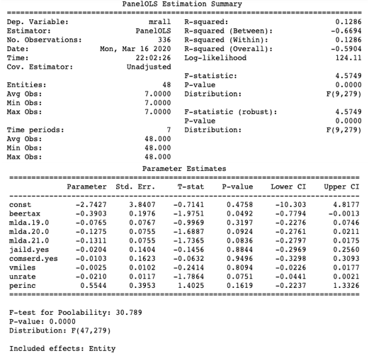
Model 2: Entity_effects

Model 2 makes the same conclusion that higher beer tax results in a lower fatality rate (the coefficient of beer tax is -0.3903).

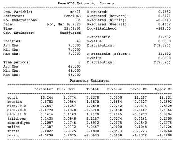
How to understand the R-squared values in the three models? The R-squared in Model 1 is 0.3577, which is higher than the R-squared 0.1286 in Model 2. This means Model 1 performs a better fit. How about 0.4662 in Model 3? Although it is much higher than those of Models 1 and 2, the pooled OLS is a misspecified model as described in the above Equation (1) and (2). Because Model 3 fails to address the endogenous issue, it cannot help us to draw causality between beer tax and the fatality rate.

Model 3: PoolOLS