
Day 25 : 60 days of Data Science and Machine Learning Series
Classification Project 2 ( part 2)..

This is the part 2 of the Classification Project 2. You can find the part 1 here :
Some of the other best Series —
100 days : Your Data Science and Machine Learning Degree Series with projects
Complete Data Visualization and Pre-processing Series with projects
Projects Videos —
All the projects, data structures, SQL, algorithms, system design, Data Science and ML , Data Analytics, Data Engineering, , Implemented Data Science and ML projects, Implemented Data Engineering Projects, Implemented Deep Learning Projects, Implemented Machine Learning Ops Projects, Implemented Time Series Analysis and Forecasting Projects, Implemented Applied Machine Learning Projects, Implemented Tensorflow and Keras Projects, Implemented PyTorch Projects, Implemented Scikit Learn Projects, Implemented Big Data Projects, Implemented Cloud Machine Learning Projects, Implemented Neural Networks Projects, Implemented OpenCV Projects,Complete ML Research Papers Summarized, Implemented Data Analytics projects, Implemented Data Visualization Projects, Implemented Data Mining Projects, Implemented Natural Leaning Processing Projects, MLOps and Deep Learning, Applied Machine Learning with Projects Series, PyTorch with Projects Series, Tensorflow and Keras with Projects Series, Scikit Learn Series with Projects, Time Series Analysis and Forecasting with Projects Series, ML System Design Case Studies Series videos will be published on our youtube channel ( just launched).
Subscribe today!
Tech Newsletter —
If you are interested, you can join my newsletter through which I send tech interview tips, techniques, patterns, hacks — Software Development, ML, Data Science, Startups and Technology projects to more than 30K readers. You can subscribe to Tech Brew :
You can get the dataset for this project here :
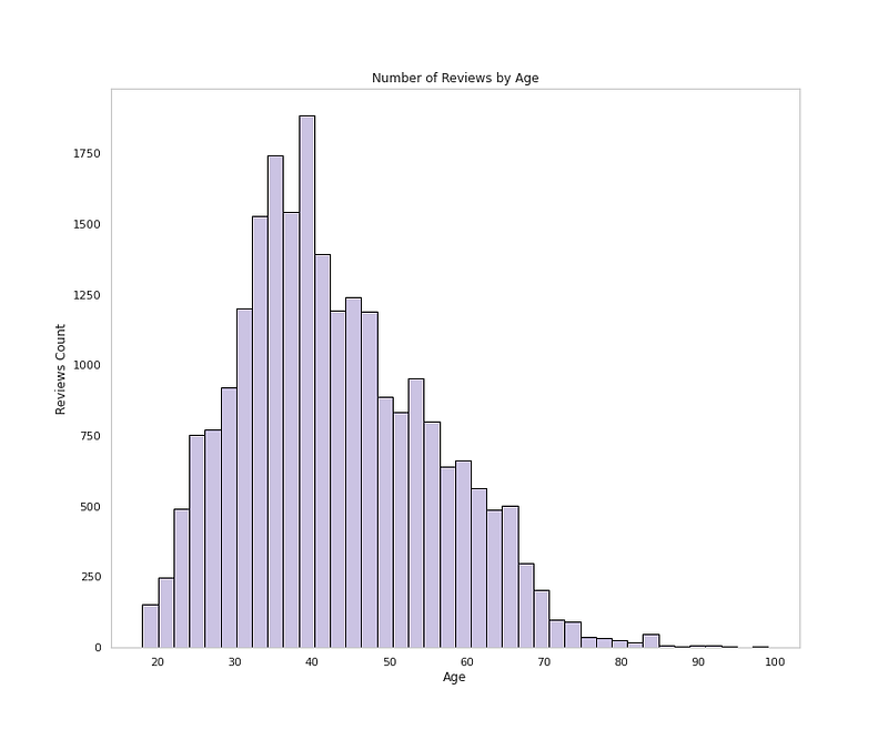
# Age Distributionplt.figure(figsize=(12,10))plt.hist(df['Age'], bins=40,color='#CBC3E3',edgecolor='black')
plt.xlabel('Age')
plt.ylabel('Reviews Count')
plt.grid(False)
plt.title('Number of Reviews by Age')
plt.show()Output —
Load the data
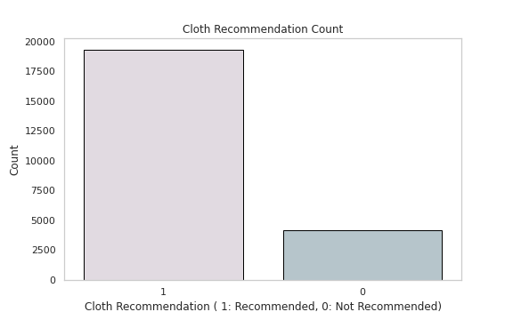
# Cloth Recommendation Analysisdf['Recommended IND'].value_counts()Output —
1    19293
0     4172
Name: Recommended IND, dtype: int64
# Cloth Recommendation Countplt.figure(figsize=(8,5))
sns.countplot(x='Recommended IND',data=df,palette=colors1,order=df['Recommended IND'].value_counts().index,edgecolor='black',linewidth=1)
plt.xlabel('Cloth Recommendation ( 1: Recommended, 0: Not Recommended)')
plt.ylabel('Count')plt.title('Cloth Recommendation Count')
plt.grid(False)
plt.show()Output —
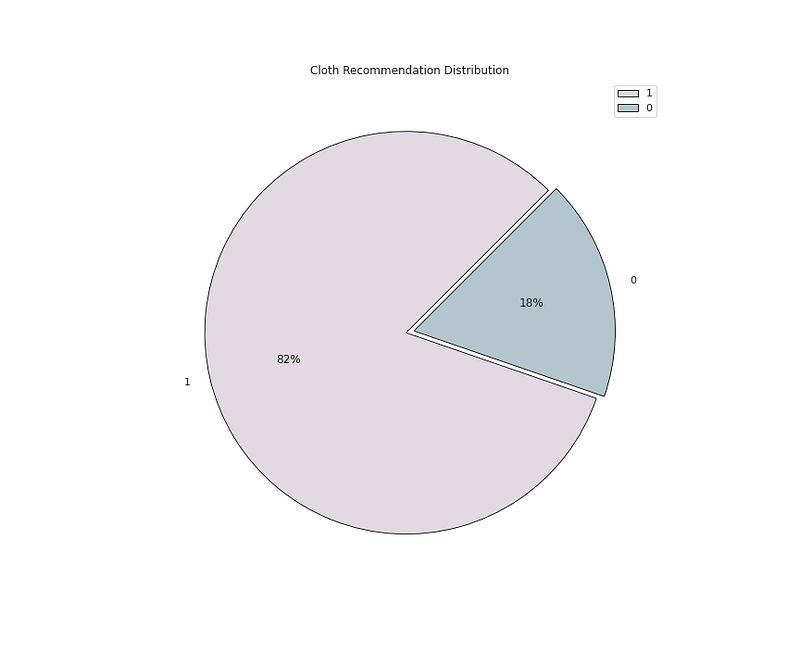
# Recommendation Distribution ( 1 means recommended and 0 means not # Recommended by the Customer)plt.figure(figsize=(12,10))
plt.pie(x=df['Recommended IND'].value_counts().values,data=df,colors=colors1,labels=df['Recommended IND'].value_counts().index,autopct='%.0f%%',explode=[0.02 for i in df['Recommended IND'].value_counts().index],startangle=45,wedgeprops={'linewidth':0.8,'edgecolor':'black'})
plt.title('Cloth Recommendation Distribution')
plt.legend()
plt.show()Output —
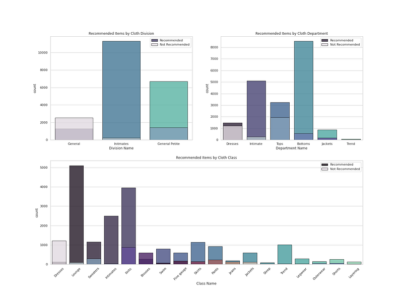
# recommendation Analysis ( 1 means recommended and 0 means not Recommended by the Customer)r = df[df['Recommended IND']==1]
not_r= df[df['Recommended IND']==0]# Plot Cloth Recommendation by Cloth Department, Division, Classfig = plt.figure(figsize=(20, 15))
ax1 = plt.subplot2grid((2, 2), (0, 0))
ax1 = sns.countplot(r['Division Name'], palette ='mako', alpha = 0.8, label = "Recommended",edgecolor='black',linewidth=1)
ax1 = sns.countplot(not_r['Division Name'], palette = colors1, alpha = 0.8, label = "Not Recommended",edgecolor='black',linewidth=1)
ax1 = plt.title("Recommended Items by Cloth Division")
ax1 = plt.legend()ax2 = plt.subplot2grid((2, 2), (0, 1))
ax2 = sns.countplot(r['Department Name'], palette ='mako', alpha = 0.8, label = "Recommended",edgecolor='black',linewidth=1)
ax2 = sns.countplot(not_r['Department Name'], palette =colors1, alpha = 0.8, label = "Not Recommended",edgecolor='black',linewidth=1)
ax2 = plt.title("Recommended Items by Cloth Department")
ax2 = plt.legend()ax3 = plt.subplot2grid((2, 2), (1, 0), colspan=2)
ax3 = plt.xticks(rotation=45)
ax3 = sns.countplot(r['Class Name'], palette ='mako', alpha = 0.8, label = "Recommended",edgecolor='black',linewidth=1)
ax3 = sns.countplot(not_r['Class Name'], palette =colors1, alpha = 0.8, label = "Not Recommended",edgecolor='black',linewidth=1)
ax3 = plt.title("Recommended Items by Cloth Class")
ax3 = plt.legend()plt.show()Output —
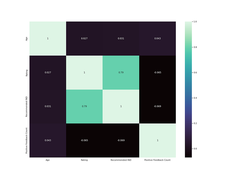
# heatmapplt.figure(figsize=(8,6))
h = df.drop('Clothing ID',axis=1).corr()
sns.heatmap(h,annot=True,cmap='mako')
plt.show()Output —
# Tokenizing the reviewsdef tokens(words):
words = re.sub("[^a-zA-Z]"," ", words)
text = words.lower().split()
return " ".join(text)
df['Review Text'] = df['Review Text'].astype(str)
df['Final_Reviews'] = df['Review Text'].apply(tokens)# Use the Stop wordssw = stopwords.words('english')clothes =['skirt','pants','white','black','fabric','silky','leather','blouse','sleeve','even','jacket','dress','color','wear','top','sweater','material','shirt','jeans','pant']
def stopwords(review):
text = [word.lower() for word in review.split() if word.lower() not in sw and word.lower() not in clothes]
return " ".join(text)
df['Final_Reviews'] = df['Final_Reviews'].apply(stopwords)# Lemmatize
from nltk.stem.wordnet import WordNetLemmatizer
lm = WordNetLemmatizer()def lemma(text):
lem_text = [lm.lemmatize(word) for word in text.split()]
return " ".join(lem_text)
df['Final_Reviews'] = df['Final_Reviews'].apply(lemma)
# Seperating Positive and Negative Reviewsnw = []
pw =[]
pos = df[df['Recommended IND']== 1]
neg = df[df['Recommended IND']== 0]for r in neg.Final_Reviews:
nw.append(r)
nw = ' '.join(nw)for r in pos.Final_Reviews:
pw.append(r)
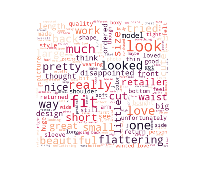
pw = ' '.join(pw)# Wordcloud of Negative Reivewswordcloud = WordCloud(background_color="white", max_words=len(nw),width=500, height=480, max_font_size=60, min_font_size=10,colormap='rocket')wordcloud.generate(nw)plt.figure(figsize=(20,17))
plt.imshow(wordcloud, interpolation="bilinear")
plt.axis("off")
plt.margins(x=0, y=0)
plt.show()Output —
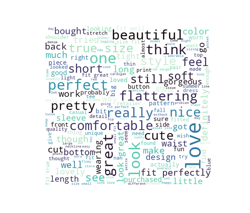
# Word Cloud of positive Reviewswordcloud = WordCloud(background_color="white", max_words=len(pw),width=500, height=480, max_font_size=60, min_font_size=10,colormap='mako')wordcloud.generate(pw)plt.figure(figsize=(20,17))
plt.imshow(wordcloud, interpolation="bilinear")
plt.axis("off")
plt.margins(x=0, y=0)
plt.show()Output —
# Building ModelX = pos['Final_Reviews']
y = pos['Recommended IND']X_train, X_test, y_train, y_test = train_test_split(X, y, test_size=0.3, random_state = 42)# Count Vectorizerv = CountVectorizer(min_df=7, ngram_range=(1,2)).fit(X_train)
X_tv = v.transform(X_train)Naive Bayes —
These are classification algorithms based on Bayes’ Theorem. They are extremely fast for both training and prediction and provide probabilistic prediction. Multinomial NB is used for discrete counts.
The formula for Bayes’ theorem is given as:
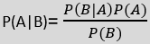
Bayes’s theorem tells us how to express this in terms of quantities we can calculate more directly:
P(L | features)=P(features | L)P(L)P(features)
Examples include spam filtration, Sentimental analysis, and classifying articles.
# Naive Bayesmodel_nb = Pipeline([('v', CountVectorizer(min_df=7, ngram_range=(1,2))),('tfidf', TfidfTransformer()),('clf',MultinomialNB())])model_nb.fit(X_train, y_train)ytest = np.array(y_test)
pred_nb = model_nb.predict(X_test)
print('accuracy %s' % accuracy_score(pred_nb, y_test))
print('Confusion Matrix:',confusion_matrix(y_test, pred_nb))
print(classification_report(ytest, pred_y))Output —
accuracy 1.0
Confusion Matrix: [[5788]]
              precision    recall  f1-score   support

           1       1.00      1.00      1.00      5788

    accuracy                           1.00      5788
   macro avg       1.00      1.00      1.00      5788
weighted avg       1.00      1.00      1.00      5788
Random Forest —
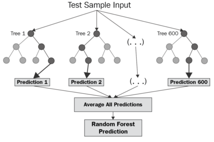
It’s a supervised machine learning algorithm that is constructed from decision tree algorithms ( it predicts the outcome by taking the average or mean of the output from the different trees) and Is used to solve both regression and classification problems. It mainly used ensemble learning, a technique in which many classifiers are combined together to provide solutions to complex problems. It’s very efficient as it reduces the overfitting of datasets, provides an effective way of handling missing data, runs efficiently on large databases, achieves extremely high accuracies, increases precision and scales really well when new features are added to the dataset..
# Random Forestmodel_rf = Pipeline([('v', CountVectorizer(min_df=7, ngram_range=(1,2))),('tfidf', TfidfTransformer()),('clf-rf', RandomForestClassifier(n_estimators=30)),])model_rf.fit(X_train, y_train)ytest = np.array(y_test)
pred_rf = model_rf.predict(X_test)
print('accuracy %s' % accuracy_score(pred_rf, y_test))
print('Confusion Matrix:', confusion_matrix(y_test, pred_rf))
print(classification_report(ytest, pred))Output —
accuracy 1.0
Confusion Matrix: [[5788]]
              precision    recall  f1-score   support

           1       1.00      1.00      1.00      5788

    accuracy                           1.00      5788
   macro avg       1.00      1.00      1.00      5788
weighted avg       1.00      1.00      1.00      5788
Day 26 : Clustering with a project!
Follow and Stay tuned.
For other projects, tune to —
Build Machine Learning Pipelines( With Code)
Recurrent Neural Network with Keras
Clustering Geolocation Data in Python using DBSCAN and K-Means
Facial Expression Recognition using Keras
Hyperparameter Tuning with Keras Tuner
Custom Layers in Keras
That’s it fellas. Peace out and keep coding :)
Stay Tuned and of-course let me end this post with a quote by Vincent Gogh
“The beginning is perhaps more difficult than anything else, but keep heart, it will turn out all right.”


