Transfer Learning for Text Classification Using PyTorch

Fine-tuning a pretrained transformer BERT model for customized sentiment analysis using PyTorch training loops

Hugging Face provides three ways to fine-tune a pretrained text classification model: PyTorch, Tensorflow Keras, and transformer trainer. Compared with the other two ways, PyTorch training loops provide more customization and easier debugging of the training loops. This tutorial will use PyTorch to fine-tune a text classification model. We will talk about the following:

• How does transfer learning work?
• How to convert a pandas dataframe into a Hugging Face Dataset?
• How to tokenize text, load a pretrained model, and train a transfer learning model using PyTorch training loops?
• How to make predictions and evaluate the model performance of a fine-tuned transfer learning model for text classification?
• How to save the model and re-load the model?

If you are interested in learning how to implement transfer Learning Using Tensorflow or transformer trainer, please check out my previous tutorial Customized Sentiment Analysis: Transfer Learning Using Tensorflow with Hugging Face and Transfer Learning for Text Classification Using Hugging Face Transformers Trainer.

Resources for this post:

• Video tutorial for this post on YouTube
• Click here for the Colab notebook
• More video tutorials on NLP
• More blog posts on NLP

Let’s get started!

Step 0: Transfer Learning Algorithms

In step 0, we will talk about how transfer learning works.

Transfer learning is a machine learning technique that reuses a pretrained large deep learning model on a new task. It usually includes the following steps:

1. Select a pretrained model that is suitable for the new task. For example, if the new task includes text from different languages, a multi-language pretrained model needs to be selected.
2. Keep all the weights and biases from the pretrained model except for the output layer. This is because the output layer for the pretrained model is for the pretrained tasks and it needs to be replaced with the new task.
3. Feed randomly initialize weights and biases into the new head of the new task. For a sentiment analysis transfer learning (aka fine-tuning) model on a pretrained BERT model, we will remove the head that classifies mask words, and replace it with the two sentiment analysis labels, positive and negative.
4. Retrain the model for the new task with the new data, utilizing the pretrained weights and biases. Because the weights and biases store the knowledge learned from the pretrained model, the fine-tuned transfer learning model can build on that knowledge and does not need to learn from scratch.

Step 1: Install And Import Python Libraries

In step 1, we will install and import python libraries.

Firstly, let’s install transformers, datasets, and evaluate.

# Install libraries
!pip install transformers datasets evaluate

After installing the python packages, we will import the python libraries.

• pandas and numpy are imported for data processing.
• torch and transformers are imported for modeling.
• tqdm is for tracking the modeling progress.
• Dataset is imported for the Hugging Face dataset format.
• evaluate is imported for model performance evaluation.

# Data processing
import pandas as pd
import numpy as np

# Modeling
import torch
from torch.utils.data import DataLoader
from torch.optim import AdamW
from transformers import AutoTokenizer, AutoModelForSequenceClassification, get_scheduler

# Progress bar
from tqdm.auto import tqdm

# Hugging Face Dataset
from datasets import Dataset

# Model performance evaluation
import evaluate

Step 2: Download And Read Data

The second step is to download and read the dataset.

The UCI Machine Learning Repository has the review data from three websites: imdb.com, amazon.com, and yelp.com. We will use the review data from amazon.com for this tutorial. Please follow these steps to download the data.

1. Go to: https://archive.ics.uci.edu/ml/datasets/Sentiment+Labelled+Sentences
2. Click “Data Folder”
3. Download “sentiment labeled sentences.zip”
4. Unzip “sentiment labeled sentences.zip”
5. Copy the file “amazon_cells_labelled.txt” to your project folder

Those who are using Google Colab for this analysis need to mount Google Drive to read the dataset. You can ignore the code below if you are not using Google Colab.

• drive.mount is used to mount to the Google drive so the colab notebook can access the data on the Google drive.
• os.chdir is used to change the default directory on Google drive. I set the default directory to the folder where the review dataset is saved.
• !pwd is used to print the current working directory.

Please check out Google Colab Tutorial for Beginners for details about using Google Colab for data science projects.

# Mount Google Drive
from google.colab import drive
drive.mount('/content/drive')

# Change directory
import os
os.chdir("drive/My Drive/contents/nlp")

# Print out the current directory
!pwd

Now let’s read the data into a pandas dataframe and see what the dataset looks like.

The dataset has two columns. One column contains the reviews and the other column contains the sentiment label for the review.

# Read in data
amz_review = pd.read_csv('sentiment labelled sentences/amazon_cells_labelled.txt', sep='\t', names=['review', 'label'])

# Take a look at the data
amz_review.head()

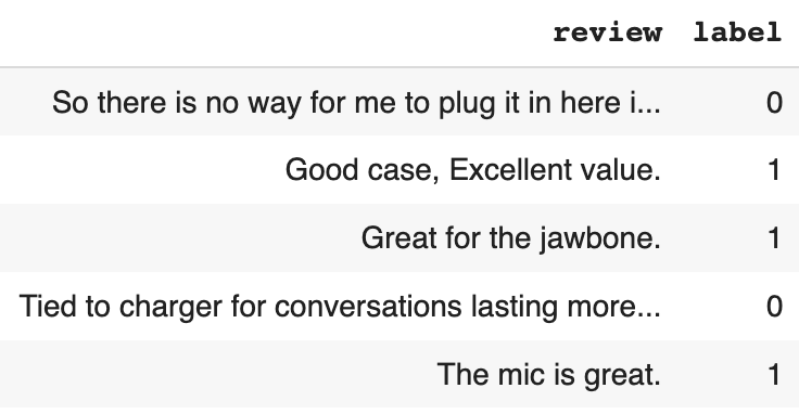
.info helps us to get information about the dataset.

# Get the dataset information
amz_review.info()

From the output, we can see that this data set has 1000 records and no missing data. The review column is the object type and the label column is the int64 type.

<class 'pandas.core.frame.DataFrame'>
RangeIndex: 1000 entries, 0 to 999
Data columns (total 2 columns):
 #   Column  Non-Null Count  Dtype 
---  ------  --------------  ----- 
 0   review  1000 non-null   object
 1   label   1000 non-null   int64 
dtypes: int64(1), object(1)
memory usage: 15.8+ KB

The label value of 0 represents negative reviews and the label value of 1 represents positive reviews. The dataset has 500 positive reviews and 500 negative reviews. It is well-balanced, so we can use accuracy as the metric to evaluate the model performance.

# Check the label distribution
amz_review['label'].value_counts()

Output:

0    500
1    500
Name: label, dtype: int64

Step 3: Train Test Split

In step 3, we will split the dataset and have 80% as the training dataset and 20% as the testing dataset.

Using the sample method, we set frac=0.8, which randomly samples 80% of the data. random_state=42 ensures that the sampling result is reproducible.

Dropping the train_data from the review dataset gives us the rest 20% of the data, which is our testing dataset.

# Training dataset
train_data = amz_review.sample(frac=0.8, random_state=42)

# Testing dataset
test_data = amz_review.drop(train_data.index)

# Check the number of records in training and testing dataset.
print(f'The training dataset has {len(train_data)} records.')
print(f'The testing dataset has {len(test_data)} records.')

After the train test split, there are 800 reviews in the training dataset and 200 reviews in the testing dataset.

The training dataset has 800 records.
The testing dataset has 200 records.

Step 4: Convert Pandas Dataframe to Hugging Face Dataset

In step 4, the training and the testing datasets will be converted from pandas dataframe to Hugging Face Dataset format.

Hugging Face Dataset objects are memory-mapped on the drive, so they are not limited by RAM memory, which is very helpful for processing large datasets.

We use Dataset.from_pandas to convert a pandas dataframe to a Hugging Face Dataset.

# Convert pyhton dataframe to Hugging Face arrow dataset
hg_train_data = Dataset.from_pandas(train_data)
hg_test_data = Dataset.from_pandas(test_data)

The length of the Hugging Face Dataset is the same as the number of records in the pandas dataframe. For example, there are 800 records in the pandas dataframe for the training dataset, and the length of the converted Hugging Face Dataset for the training dataset is 800 too.

hg_train_data[0] gives us the first record in the Hugging Face Dataset. It is a dictionary with three keys, review, label, and __index_level_0__.

• review is the variable name for the review text. The name is inherited from the column name of the pandas dataframe.
• label is the variable name for the sentiment of the review text. The name is inherited from the column name of the pandas dataframe too.
• __index_level_0__ is an automatically generated field from the pandas dataframe. It stores the index of the corresponding record.

# Length of the Dataset
print(f'The length of hg_train_data is {len(hg_train_data)}.\n')

# Check one review
hg_train_data[0]

In this example, we can see that the review is Thanks again to Amazon for having the things I need for a good price!, the sentiment for the review is positive/1, and the index of this record is 521 in the pandas dataframe.

The length of hg_train_data is 800.

{'review': 'Thanks again to Amazon for having the things I need for a good price!',
 'label': 1,
 '__index_level_0__': 521}

Checking the index 521 in the pandas dataframe confirms the same information with Hugging Face Dataset.

# Validate the record in pandas dataframe
amz_review.iloc[[521]]

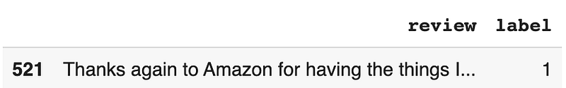
Step 5: Tokenize Text

In step 5, we will tokenize the review text using a tokenizer.

A tokenizer converts text into numbers to use as the input of the NLP (Natural Language Processing) models. Each number represents a token, which can be a word, part of a word, punctuation, or special tokens. How the text is tokenized is determined by the pretrained model. AutoTokenizer.from_pretrained("bert-base-cased") is used to download vocabulary from the pretrained bert-base-cased model, meaning that the text will be tokenized like a BERT model.

# Tokenizer from a pretrained model
tokenizer = AutoTokenizer.from_pretrained("bert-base-cased")

# Take a look at the tokenizer
tokenizer

We can see that the tokenizer contains information such as model name, vocabulary size, max length, padding position, truncation position, and special tokens.

BertTokenizerFast(name_or_path='bert-base-cased', vocab_size=28996, model_max_length=512, is_fast=True, padding_side='right', truncation_side='right', special_tokens={'unk_token': '[UNK]', 'sep_token': '[SEP]', 'pad_token': '[PAD]', 'cls_token': '[CLS]', 'mask_token': '[MASK]'})

There are five special tokens for the BERT model. Other models may have different special tokens.

• The tokens that are not part of the BERT model training dataset are unknown tokens. The unknown token is [UNK] and the ID for the unknown token is 100.
• The separator token is [SEP] and the ID for the separator token is 102.
• The pad token is [PAD] and the ID for the pad token is 0.
• The sentence level classification token is [CLS] and the ID for the classification token is 101.
• The mask token is [MASK] and the ID for the mask token is 103.

# Mapping between special tokens and their IDs.
print(f'The unknown token is {tokenizer.unk_token} and the ID for the unkown token is {tokenizer.unk_token_id}.')
print(f'The seperator token is {tokenizer.sep_token} and the ID for the seperator token is {tokenizer.sep_token_id}.')
print(f'The pad token is {tokenizer.pad_token} and the ID for the pad token is {tokenizer.pad_token_id}.')
print(f'The sentence level classification token is {tokenizer.cls_token} and the ID for the classification token is {tokenizer.cls_token_id}.')
print(f'The mask token is {tokenizer.mask_token} and the ID for the mask token is {tokenizer.mask_token_id}.')

Output:

The unknown token is [UNK] and the ID for the unkown token is 100.
The seperator token is [SEP] and the ID for the seperator token is 102.
The pad token is [PAD] and the ID for the pad token is 0.
The sentence level classification token is [CLS] and the ID for the classification token is 101.
The mask token is [MASK] and the ID for the mask token is 103.

After downloading the model vocabulary, the method tokenizer is used to tokenize the review corpus.

• max_length indicates the maximum number of tokens kept for each document.

👉 If the document has more tokens than the max_length, it will be truncated.

👉 If the document has less tokens than the max_length, it will be padded with zeros.

👉 If max_length is unset or set to None, the maximum length from the pretrained model will be used. If the pretrained model does not have a maximum length parameter, max_length will be deactivated.

• truncation controls how the token truncation is implemented. truncation=True indicates that the truncation length is the length specified by max_length. If max_length is not specified, the max_length of the pretrained model is used.
• padding means adding zeros to shorter reviews in the dataset. The padding argument controls how padding is conducted.

👉 padding=True is the same as padding='longest'. It checks the longest sequence in the batch and pads zeros to that length. There is no padding if only one text document is provided.

👉 padding='max_length' pads to max_length if it is specified, otherwise, it pads to the maximum acceptable input length for the model.

👉 padding=False is the same as padding='do_not_pad'. It is the default, indicating that no padding is applied, so it can output a batch with sequences of different lengths.

# Funtion to tokenize data
def tokenize_dataset(data):
    return tokenizer(data["review"], 
                     max_length=32, 
                     truncation=True, 
                     padding="max_length")

# Tokenize the dataset
dataset_train = hg_train_data.map(tokenize_dataset)
dataset_test = hg_test_data.map(tokenize_dataset)

After tokenization, we can see that both the training and the testing Dataset have 6 features, 'review', 'label', '__index_level_0__', 'input_ids', 'token_type_ids', and 'attention_mask'. The number of rows is stored with num_rows.

# Take a look at the data
print(dataset_train)
print(dataset_test)

Output:

Dataset({
    features: ['review', 'label', '__index_level_0__', 'input_ids', 'token_type_ids', 'attention_mask'],
    num_rows: 800
})
Dataset({
    features: ['review', 'label', '__index_level_0__', 'input_ids', 'token_type_ids', 'attention_mask'],
    num_rows: 200
})

Next, some data processing is needed to make the training and testing datasets compatible with the model.

• "review" and "__index_level_0__" are removed because they will not be used in the model.
• "label" is renamed to "labels" because the model expects the name "labels".
• The format of the datasets is set to PyTorch tensors.

# Remove the review and index columns because it will not be used in the model
dataset_train = dataset_train.remove_columns(["review", "__index_level_0__"])
dataset_test = dataset_test.remove_columns(["review", "__index_level_0__"])

# Rename label to labels because the model expects the name labels
dataset_train = dataset_train.rename_column("label", "labels")
dataset_test = dataset_test.rename_column("label", "labels")

# Change the format to PyTorch tensors
dataset_train.set_format("torch")
dataset_test.set_format("torch")

# Take a look at the data
print(dataset_train)
print(dataset_test)

After the data processing, we can see that both training and testing datasets have four features.

Dataset({
    features: ['labels', 'input_ids', 'token_type_ids', 'attention_mask'],
    num_rows: 800
})
Dataset({
    features: ['labels', 'input_ids', 'token_type_ids', 'attention_mask'],
    num_rows: 200
})

dataset_train[0] gives us the content for the first record in the training dataset in a dictionary format.

• 'labels' is the label of the classification. The first record is a positive review, so the label is 1.
• 'input_ids' are the IDs for the tokens. There are 32 token IDs because the max_length is 32 for the tokenization.
• 'token_type_ids' is also called segment IDs.

👉 BERT was trained on two tasks, Masked Language Modeling and Next Sentence Prediction. 'token_type_ids' is for the Next Sentence Prediction, where two sentences are used to predict whether the second sentence is the next sentence for the first one.

👉 The first sentence has all the tokens represented by zeros, and the second sentence has all the tokens represented by ones.

👉 Because our classification task does not have a second sentence, all the values for 'token_type_ids' are zeros.

• 'attention_mask' indicates which token ID should get attention from the model, so the padding tokens are all zeros and other tokens are 1s.

# Check the first record
dataset_train[0]

Output:

{'labels': tensor(1),
 'input_ids': tensor([ 101, 5749, 1254, 1106, 9786, 1111, 1515, 1103, 1614,  146, 1444, 1111,
          170, 1363, 3945,  106,  102,    0,    0,    0,    0,    0,    0,    0,
            0,    0,    0,    0,    0,    0,    0,    0]),
 'token_type_ids': tensor([0, 0, 0, 0, 0, 0, 0, 0, 0, 0, 0, 0, 0, 0, 0, 0, 0, 0, 0, 0, 0, 0, 0, 0,
         0, 0, 0, 0, 0, 0, 0, 0]),
 'attention_mask': tensor([1, 1, 1, 1, 1, 1, 1, 1, 1, 1, 1, 1, 1, 1, 1, 1, 1, 0, 0, 0, 0, 0, 0, 0,
         0, 0, 0, 0, 0, 0, 0, 0])}

Step 6: DataLoader

In step 6, we will put the training and testing datasets into DataLoader.

DataLoader is a parallel data loading process by PyTorch. It increases the data loading speed and decreases memory usage.

• dataset takes the dataset name to put in the DataLoader.
• shuffle=True indicates that the data will be reshuffled at every epoch. The default value is False. We set it True for the training dataset and keep the default False for the testing dataset.
• batch_size=4 means that 4 samples will be loaded for each batch. The default value is 1.

Before putting the dataset into DataLoader, the unoccupied cached memory is released by torch.cuda.empty_cache().

# Empty cache
torch.cuda.empty_cache()

# DataLoader
train_dataloader = DataLoader(dataset=dataset_train, shuffle=True, batch_size=4)
eval_dataloader = DataLoader(dataset=dataset_test, batch_size=4)

Step 7: Load Pretrained Model

In step 7, we will load the pretrained model for sentiment analysis.

• AutoModelForSequenceClassification loads the BERT model without the sequence classification head.
• The method from_pretrained() loads the weights from the pretrained model into the new model, so the weights in the new model are not randomly initialized. Note that the new weights for the new sequence classification head are going to be randomly initialized.
• bert-base-cased is the name of the pretrained model. We can change it to a different model based on the nature of the project.
• num_labels indicates the number of classes. Our dataset has two classes, positive and negative, so num_labels=2.

# Load model
model = AutoModelForSequenceClassification.from_pretrained("bert-base-cased", num_labels=2)

Step 8: Set Learning Rate Scheduler

In step 8, we will set up the learning rate scheduler using the get_scheduler method.

• name="linear" indicates that the name of the scheduler is linear.
• optimizer takes AdamW as the optimizer. AdamW is a variation of the Adam optimizer. It modifies the weight decay in Adam by decoupling weight decay from the gradient update. params takes the model parameters. lr is the learning rate.
• num_warmup_steps=0 indicates that there are no warmup steps.
• num_training_steps is the number of training steps. It is calculated as the number of epochs times the number of batches. We set the number of epochs to be 2, meaning that the model will go through the whole training dataset 2 times. The number of batches is the length of the training data loader.

Then we set the model to use GPU if it is available.

# Number of epochs
num_epochs = 2

# Number of training steps
num_training_steps = num_epochs * len(train_dataloader)

# Optimizer
optimizer = AdamW(params=model.parameters(), lr=5e-6)

# Set up the learning rate scheduler
lr_scheduler = get_scheduler(name="linear", 
                             optimizer=optimizer, 
                             num_warmup_steps=0, 
                             num_training_steps=num_training_steps)

# Use GPU if it is available
device = torch.device("cuda") if torch.cuda.is_available() else torch.device("cpu")
model.to(device)

Step 9: PyTorch Training Loop

In step 9, we will run the PyTorch training loop for the transfer learning model.

model.train() tells the model that we are training the model. Some layers work differently for training and evaluation, and model.train() helps to inform the layers that the model training is in progress.

Then the PyTorch training loop runs through each batch for each epoch.

• Firstly, the data is fetched from the batch and passed into the model.
• Then, the output of the model is used to calculate the loss and update the weights based on backpropagation results.
• After that, the learning rate scheduler is executed and the gradients are cleared.
• Finally, the progress bar is updated to reflect the training progress.

# Set the progress bar
progress_bar = tqdm(range(num_training_steps))

# Tells the model that we are training the model
model.train()
# Loop through the epochs
for epoch in range(num_epochs):
    # Loop through the batches
    for batch in train_dataloader:
        # Get the batch
        batch = {k: v.to(device) for k, v in batch.items()}
        # Compute the model output for the batch
        outputs = model(**batch)
        # Loss computed by the model
        loss = outputs.loss
        # backpropagates the error to calculate gradients
        loss.backward()
        # Update the model weights
        optimizer.step()
        # Learning rate scheduler
        lr_scheduler.step()
        # Clear the gradients
        optimizer.zero_grad()
        # Update the progress bar
        progress_bar.update(1)

Step 10: PyTorch Model Prediction and Evaluation

In step 10, we will talk about how to make model predictions and evaluations using PyTorch.

Hugging Face has an evaluate library with over 100 evaluation modules. We can see the list of all the modules using evaluate.list_evaluation_modules().

# Number of evaluation modules
print(f'There are {len(evaluate.list_evaluation_modules())} evaluation models in Hugging Face.\n')

# List all evaluation metrics
evaluate.list_evaluation_modules()

Output:

There are 129 evaluation models in Hugging Face.

['lvwerra/test',
 'precision',
 'code_eval',
 'roc_auc',
 'cuad',
 'xnli',
 'rouge',
 'pearsonr',
 'mse',
 'super_glue',
 'comet',
 'cer',
 'sacrebleu',
 'mahalanobis',
 'wer',
 'competition_math',
 'f1',
 'recall',
 'coval',
 'mauve',
 'xtreme_s',
 'bleurt',
 'ter',
 'accuracy',
 'exact_match',
 'indic_glue',
 'spearmanr',
 'mae',
 'squad',
 'chrf',
 'glue',
 'perplexity',
 'mean_iou',
 'squad_v2',
 'meteor',
 'bleu',
 'wiki_split',
 'sari',
 'frugalscore',
 'google_bleu',
 'bertscore',
 'matthews_correlation',
 'seqeval',
 'trec_eval',
 'rl_reliability',
 'jordyvl/ece',
 'angelina-wang/directional_bias_amplification',
 'cpllab/syntaxgym',
 'lvwerra/bary_score',
 'kaggle/amex',
 'kaggle/ai4code',
 'hack/test_metric',
 'yzha/ctc_eval',
 'codeparrot/apps_metric',
 'mfumanelli/geometric_mean',
 'daiyizheng/valid',
 'poseval',
 'erntkn/dice_coefficient',
 'mgfrantz/roc_auc_macro',
 'Vlasta/pr_auc',
 'gorkaartola/metric_for_tp_fp_samples',
 'idsedykh/metric',
 'idsedykh/codebleu2',
 'idsedykh/codebleu',
 'idsedykh/megaglue',
 'kasmith/woodscore',
 'cakiki/ndcg',
 'brier_score',
 'Vertaix/vendiscore',
 'GMFTBY/dailydialogevaluate',
 'GMFTBY/dailydialog_evaluate',
 'jzm-mailchimp/joshs_second_test_metric',
 'ola13/precision_at_k',
 'yulong-me/yl_metric',
 'abidlabs/mean_iou',
 'abidlabs/mean_iou2',
 'KevinSpaghetti/accuracyk',
 'Felipehonorato/my_metric',
 'NimaBoscarino/weat',
 'ronaldahmed/nwentfaithfulness',
 'Viona/infolm',
 'kyokote/my_metric2',
 'kashif/mape',
 'Ochiroo/rouge_mn',
 'giulio98/code_eval_outputs',
 'leslyarun/fbeta_score',
 'giulio98/codebleu',
 'anz2/iliauniiccocrevaluation',
 'zbeloki/m2',
 'xu1998hz/sescore',
 'mase',
 'mape',
 'smape',
 'dvitel/codebleu',
 'NCSOFT/harim_plus',
 'JP-SystemsX/nDCG',
 'sportlosos/sescore',
 'Drunper/metrica_tesi',
 'jpxkqx/peak_signal_to_noise_ratio',
 'jpxkqx/signal_to_reconstrution_error',
 'hpi-dhc/FairEval',
 'nist_mt',
 'lvwerra/accuracy_score',
 'character',
 'charcut_mt',
 'ybelkada/cocoevaluate',
 'harshhpareek/bertscore',
 'posicube/mean_reciprocal_rank',
 'bstrai/classification_report',
 'omidf/squad_precision_recall',
 'Josh98/nl2bash_m',
 'BucketHeadP65/confusion_matrix',
 'BucketHeadP65/roc_curve',
 'mcnemar',
 'exact_match',
 'wilcoxon',
 'ncoop57/levenshtein_distance',
 'kaleidophon/almost_stochastic_order',
 'word_length',
 'lvwerra/element_count',
 'word_count',
 'text_duplicates',
 'perplexity',
 'label_distribution',
 'toxicity',
 'prb977/cooccurrence_count',
 'regard',
 'honest',
 'NimaBoscarino/pseudo_perplexity']

We will use three metrics to evaluate the model performance. They are accuracy, f1, and recall.

• accuracy is the percentage of correct predictions. It ranges from 0 to 1, where 1 means perfect prediction. The higher value the accuracy is, the better the model is when the data is balanced.
• recall is also called sensitivity or true positive rate. It is the percentage of positive events captured out of all the positive events. The value for recall ranges from 0 to 1. The higher value the recall is, the better the model is.
• f1 is a metric that balances precision and recall values, and it should be used when there is no clear preference between precision and recall. The F1 score ranges from 0 to 1, with the best value being 1 and the worst value being 0.

# Load the evaluation metric
metric1 = evaluate.load("accuracy")
metric2 = evaluate.load("f1")
metric3 = evaluate.load("recall")

The prediction and evaluation process starts with model.eval(), which tells PyTorch that we are evaluating the model instead of training the model.

Because the model evaluation is processed in batches, empty lists are created to hold all the prediction results for logits, predicted probabilities, and predicted labels.

# Tells the model that we are evaluting the model performance
model.eval()

#  A list for all logits
logits_all = []

# A list for all predicted probabilities
predicted_prob_all = []

# A list for all predicted labels
predictions_all = []

The model predictions and evaluations are completed in the same loop for the batches. Note that since this is the prediction step, no epoch is needed.

• Firstly, we get the data from the batch and pass it to the model for prediction. torch.no_grad() is included to disable the gradient calculation. The gradient calculation is disabled for the prediction because it is only needed for the training process.
• Then logits are extracted from the prediction output and appended to the list logits_all. Logit values from all classes do not sum up to 1.
• To get the predicted probabilities, torch.softmax is applied on the logits. dim=1 means that the softmax is calculated based on the rows, so for each sample, the predicted probabilities for all classes sum up to 1.
• The label prediction can be based on either logits or predicted probabilities. In this example, we are using logits, but the predicted probabilities should give the same results. dim=-1 means that the last column is the event of interest.
• After having the predictions, the model performance metrics are calculated. references takes the true labels for the batch.

# Loop through the batches in the evaluation dataloader
for batch in eval_dataloader:
    # Get the batch
    batch = {k: v.to(device) for k, v in batch.items()}
    # Disable the gradient calculation
    with torch.no_grad():
        # Compute the model output
        outputs = model(**batch)
    # Get the logits
    logits = outputs.logits
    # Append the logits batch to the list
    logits_all.append(logits)
    # Get the predicted probabilities for the batch
    predicted_prob = torch.softmax(logits, dim=1)
    # Append the predicted probabilities for the batch to all the predicted probabilities
    predicted_prob_all.append(predicted_prob)
    # Get the predicted labels for the batch
    predictions = torch.argmax(logits, dim=-1)
    # Append the predicted labels for the batch to all the predictions
    predictions_all.append(predictions)
    # Add the prediction batch to the evaluation metric
    metric1.add_batch(predictions=predictions, references=batch["labels"])
    metric2.add_batch(predictions=predictions, references=batch["labels"])
    metric3.add_batch(predictions=predictions, references=batch["labels"])

# Compute the metric
print(metric1.compute())
print(metric2.compute())
print(metric3.compute())

The evaluation results show that the model has 0.945 accuracy, 0.943 f1 score, and 0.929 recall value.

{'accuracy': 0.945}
{'f1': 0.9430051813471502}
{'recall': 0.9285714285714286}

logits_all[:5] gives us the first 5 batches of logits. We can see that the prediction has two columns. The first column is the predicted logit for label 0 and the second column is the predicted logit for label 1. Each batch has four samples.

# Take a look at the logits
logits_all[:5]

Output:

[tensor([[-1.4175,  1.7728],
         [-1.4442,  1.8167],
         [-1.2888,  1.7954],
         [ 1.1902, -1.3435]], device='cuda:0'), tensor([[ 1.0639, -1.3628],
         [-1.3469,  1.6955],
         [ 0.8422, -1.3144],
         [ 1.1680, -1.4845]], device='cuda:0'), tensor([[-1.0588,  1.3745],
         [ 1.2833, -1.2503],
         [-1.5322,  1.5994],
         [ 0.1853, -0.6757]], device='cuda:0'), tensor([[-0.9469,  1.0366],
         [-0.8427,  1.0451],
         [-1.3804,  1.6149],
         [ 0.8212, -1.0765]], device='cuda:0'), tensor([[ 0.9545, -1.2628],
         [-1.4912,  1.8893],
         [-1.4786,  1.6621],
         [ 1.4001, -1.4412]], device='cuda:0')]

predicted_prob_all[:5] gives the first five batches of the predicted probabilities. We can see that the sum of each row adds up to 1.

# Take a look at the predicted probabilities
predicted_prob_all[:5]

[tensor([[0.0395, 0.9605],
         [0.0369, 0.9631],
         [0.0438, 0.9562],
         [0.9265, 0.0735]], device='cuda:0'), tensor([[0.9188, 0.0812],
         [0.0455, 0.9545],
         [0.8963, 0.1037],
         [0.9342, 0.0658]], device='cuda:0'), tensor([[0.0807, 0.9193],
         [0.9265, 0.0735],
         [0.0418, 0.9582],
         [0.7029, 0.2971]], device='cuda:0'), tensor([[0.1209, 0.8791],
         [0.1315, 0.8685],
         [0.0476, 0.9524],
         [0.8696, 0.1304]], device='cuda:0'), tensor([[0.9018, 0.0982],
         [0.0329, 0.9671],
         [0.0415, 0.9585],
         [0.9449, 0.0551]], device='cuda:0')]

predictions_all[:5] gives the first five batches of the predicted labels. We can see that the ones correspond to the higher value of logits and the zeros correspond to the lower value of the logits for each sample.

# Take a look at the predicted labels
predictions_all[:5]

Output:

[tensor([1, 1, 1, 0], device='cuda:0'),
 tensor([0, 1, 0, 0], device='cuda:0'),
 tensor([1, 0, 1, 0], device='cuda:0'),
 tensor([1, 1, 1, 0], device='cuda:0'),
 tensor([0, 1, 1, 0], device='cuda:0')]

Step 11: Save and Load Model

In step 11, we will talk about how to save the model and reload it for prediction.

tokenizer.save_pretrained saves the tokenizer information to the drive and model.save_model saves the model to the drive.

# Save tokenizer
tokenizer.save_pretrained('./sentiment_transfer_learning_pytorch/')

# Save model
model.save_pretrained('./sentiment_transfer_learning_pytorch/')

We can load the saved tokenizer later using AutoTokenizer.from_pretrained() and load the saved model using AutoModelForSequenceClassification.from_pretrained().

# Load tokenizer
tokenizer = AutoTokenizer.from_pretrained("./sentiment_transfer_learning_pytorch/")

# Load model
loaded_model = AutoModelForSequenceClassification.from_pretrained('./sentiment_transfer_learning_pytorch/')

More tutorials are available on GrabNGoInfo YouTube Channel, GrabNGoInfo.com, and LinkedIn.

Recommended Tutorials

• GrabNGoInfo Machine Learning Tutorials Inventory
• Transfer Learning for Text Classification Using Hugging Face Transformers Trainer
• Customized Sentiment Analysis: Transfer Learning Using Tensorflow with Hugging Face
• Sentiment Analysis: Hugging Face Zero-shot Model vs Flair Pre-trained Model
• Zero-shot Topic Modeling with Deep Learning Using Python
• Topic Modeling with Deep Learning Using Python BERTopic
• Google Colab Tutorial for Beginners
• TextBlob vs. VADER for Sentiment Analysis Using Python
• Five Ways To Create Tables In Databricks
• Time Series Anomaly Detection Using Prophet in Python
• Multivariate Time Series Forecasting with Seasonality and Holiday Effect Using Prophet in Python
• Time Series Causal Impact Analysis in Python

References

• Hugging Face documentation on fine-tuning a pretrained model
• Hugging Face notebook on fine-tuning a pretrained model
• Hugging Face documentation on tokenizer
• Deeplearning.AI transfer learning video from Andrew Ng
• Hugging Face documentation on prepare_tf_dataset()
• Hugging Face documentation on Datasets
• Decoupled Weight Decay Regularization paper