Microbial Knowledge Graph with BioCypher and SemSpect

Construct and analyze a Biolink-compatible graph

This article has been updated to reflect the newest changes in BioCypher 0.5.35.

A knowledge graph (KG) is a type of database that stores and organizes knowledge in a graph-like structure, where nodes represent entities and edges represent relationships between them. It is designed to capture complex relationships and dependencies among different pieces of information, enabling more effective search, retrieval, and analysis of data. Knowledge graphs are commonly used in biology and healthcare.

OpenAI’s GPT-3 and ChatGPT have made the construction and query of knowledge graphs a lot easier. Now, every biologist can build his or her own knowledge graphs. It is no surprise that biological knowledge graphs are popping up like mushrooms in Medium, LinkedIn, and GitHub (1, 2, 3, 4, 5, 6, 7, and 8). But there are two problems.

Firstly, many of these private knowledge graphs used non-standardized vocabulary. For example, a taxon can be called Taxon in one knowledge graph and NCBITaxon in another. As a result, it is difficult to merge knowledge graphs by different creators, and sometimes by the same creator on different projects. So bioinformaticians usually create their graphs from scratch and often reinvent the wheels.

Secondly, it is hard to interact with large knowledge graphs. Biological knowledge graphs can contain thousands and even millions of nodes and relations. Thus, it is quite challenging to visualize, filter and summarize them, especially for non-programmers.

Fortunately, there are solutions. To solve the first problem, we can label our nodes and edges based on the Biolink model. Biolink is a high-level data model of biological entities (genes, diseases, phenotypes, pathways, individuals, substances, etc.) and their associations. In other words, it is a controlled vocabulary that every graph creator should adhere to. As a consequence, it is easy to share and merge Biolink-compatible graphs. And a Python library called BioCypher can help us build such graphs.

As to the second problem, we can turn to SemSpect or Gemini. These no-code apps can filter, aggregate and summarize large amounts of graph data efficiently. With their help, users can gain quick insights into their graphs.

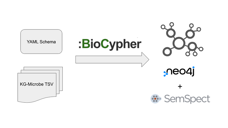
Unfortunately, there is hardly any tutorial or use case about them both outside their official website. In this article, I am going to fill this gap (Figure 1). I will use BioCypher to build a small biological knowledge graph based on the Knowledge Graphs for Microbial data (KG-Microbe). Afterward, I will gain a nice overview of the graph with SemSpect. You can find the code in my GitHub repository here.

1. The data

Knowledge Graphs for Microbial data is one of the exemplary Biolink projects (1). Its data mainly depicts the bacteria and their metabolic capacities. It shows us how biochemical pathways are shared among different bacterial lineages and, ultimately, how the bacteria evolved.

We can download and convert the data to TSV by following these instructions. The conversion didn’t work for me under Windows 11. So I turned to a Mac and finished the process. You can download my converted TSV files here.

In this project, we only need the nodes and edges from condensed_traits_NCBI and ncbitaxon.

2. Data processing and import into Neo4j 5

Next, let’s use BioCypher to generate Biolink-compatible labels for the nodes and edges. BioCypher works like this: it listens to an input data stream and formats the graph elements according to a user-defined schema into TSV. Finally, it writes us a terminal command to import the data into Neo4j.

2.1 Nodes

Here, I will demonstrate how to generate the BiologicalProcess nodes. First, the YAML schema file for the BiologicalProcess nodes looks like this.

biological process:                            # mapping
  represented_as: node              # schema configuration
  label_in_input: biolink:BiologicalProcess   # connection to input stream
  properties:
    name: st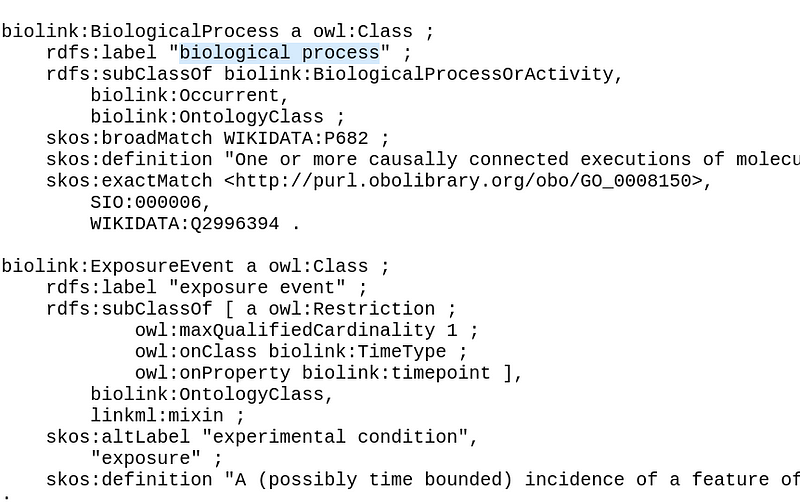r

The first line assigns our nodes to the BiologicalProcess class in Biolink. This is one of the biggest gotchas in BioCypher. For a Biolink-compatible graph, all first line must come from a rdfs:label in the biolink-model.owl.ttl file. The reason is that BioCypher will search the node class in the Biolink vocabulary. When it finds a match, BioCypher will add the parent classes to the nodes as graph labels. In other words, BioCypher generates the complete Biolink ontology for our nodes. And that can be very valuable for our analyses later. In the current BioCypher version of 0.5.35, they must be written in lower case (“biological process”). And if you let BioCypher reveal the ontology:

driver.show_ontology_structure()

you can see that all node classes are the children of the NamedThing class. The rest of the YAML is quite self-explanatory.

Next, we can write the Python script like this.

import biocypher
import pandas as pd

trait_node_file = "[PATH_TO_condensed_traits_NCBI_nodes.tsv]"

trait_nodes = pd.read_csv(trait_node_file, sep="\t")

def BiologicalProcess_generator():
    for row in trait_nodes[trait_nodes["category"] == "biolink:BiologicalProcess"].itertuples():
        yield (
          row.id,
          row.category,
          {"name": row.name}
        )

driver = biocypher.BioCypher(
    offline=True,
    schema_config_path="schema/BiologicalProcess.yaml"
)
driver.write_nodes(BiologicalProcess_generator())

driver.write_import_call()

The script reads the TSV file from KG-Microbe into a pandas data frame. A driver object reads the YAML schema and generates the node entries with its write_nodes function. This function accepts a generator (BiologicalProcess_generator) as an argument. The generator picks up lines that contain the category “biolink:BiologicalProcess” from the data frame. For each entry, the generator yields a triplet tuple. The first element is the node ID. The second element is the node category. It is noteworthy that this second value must match the label_in_input value in the YAML file. The third element is a map that contains the node properties. Finally, the write_import_call function writes the terminal command that imports the data into Neo4j.

Here comes the second gotcha. BioCypher uses the current timestamp to name the output folder. So if you carry out two consecutive write_import_call function calls within the same minute, the second terminal command will overwrite the first one. So wait at least a few seconds before the second call.

2.2 Edges

The edges are processed similarly. Let’s take the capabale_of edge as our example. The YAML file looks like this.

organism taxon to entity association:
  represented_as: edge
  source: OrganismTaxon
  target: BiologicalProcess 
  label_in_input: biolink:capable_of
  label_as_edge: capable_of

This file states that the capabale_of edge connects the taxon and its biological processes. Again, the first line must come from a rdfs:labelin the biolink-model.owl.ttl file. Line 5 states that the only lines of the biolink:capable_of categroy from the input stream are recognized. Finally, label_as_edge sets the edge label in the graph. I suggest that you get the label name from the Association list in Biolink. Be aware that BioCypher will output the label in capitalized case (“Capable_of”).

trait_edges = pd.read_csv(trait_edge_file, sep="\t")
trait_edges.head()

def capable_of_generator():
    for row in trait_edges[trait_edges["predicate"] == "biolink:capable_of"].itertuples():
        yield (
          f"{row.subject}_{row.object}",
          row.subject,
          row.object,
          row.predicate,
          {}
        )

driver = biocypher.BioCypher(
    offline=True,
    schema_config_path="schema/OrganismTaxon_BiologicalProcess.yaml"
)
driver.write_edges(capable_of_generator())
driver.write_import_call()

2.3 Data import to Neo4j 5

With the aforementioned methods, I have also created the OrganismTaxon nodes and the subclass_of edges (all the code in my GitHub repository). They are CSV files under the biocypher-out folder. Now it is time to import the data into Neo4j. At the time of writing, BioCypher does not output the correct import command for Neo4j 5. Fortunately, we can craft the command ourselves easily.

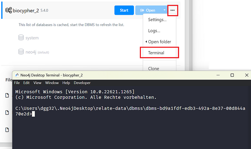
First, create a local DBMS in the Neo4j Desktop with Version 5. Then click the … button and click Terminal (Figure 3).

Adjust and execute the following command in the terminal (all in one line). On Windows, replace the “/” with “\” after “bin”.

bin/neo4j-admin database import full --delimiter=";" --array-delimiter="|" \   
--nodes="[paths_to_your_node_csv]" \
--relationships="[paths_to_your_edge_csv]" \
--quote="'" \
--overwrite-destination [database_name]

You can copy the — nodes= and — relationships= lines from your neo4j-admin-import-call.sh files generated by BioCypher. For example, my import command on Windows looks like this (all in one line).

bin/neo4j-admin database import full --delimiter=";" --array-delimiter="|" \
--nodes=/home/dgg32/Documents/kg_microbe_biocypher_semspect/biocypher-out/20240107171042/OrganismTaxon-.* \
--nodes=/home/dgg32/Documents/kg_microbe_biocypher_semspect/biocypher-out/20240107171105/BiologicalProcess-.* \
--nodes=/home/dgg32/Documents/kg_microbe_biocypher_semspect/biocypher-out/20240107171110/BiologicalProcess-.* \
--relationships=/home/dgg32/Documents/kg_microbe_biocypher_semspect/biocypher-out/20240107171116/Subclass_of-.* \
--relationships=/home/dgg32/Documents/kg_microbe_biocypher_semspect/biocypher-out/20240107171139/Capable_of-.* \
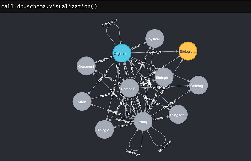
--quote="'" --overwrite-destination neo4j

Afterward, all the data will be inside your Neo4j project. You can do a quick check by calling the schema in the Neo4j Browser.

call db.schema.visualization()

And the result looks like Figure 4.

3. Data analysis with SemSpect

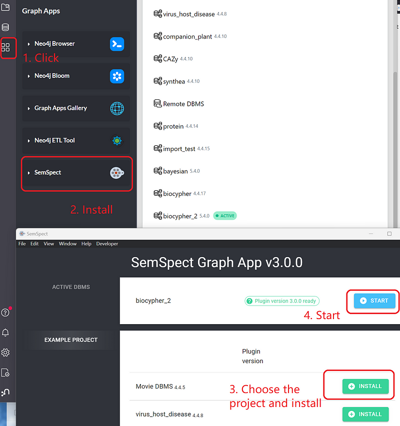
Neo4j Desktop and Bloom are powerful. But they are not exactly no-code solutions. For non-programmers, SemSpect is a good starting point for some initial data exploration. This Neo4j graph app is developed by derivo. You can install it on the Graph Apps panel in the Neo4j Desktop and then add it to your project (Figure 5).

SemSpect has a free and a PRO version. The PRO version gives you access to its Explorations and SemSpect labels features. But even the free version is very powerful.

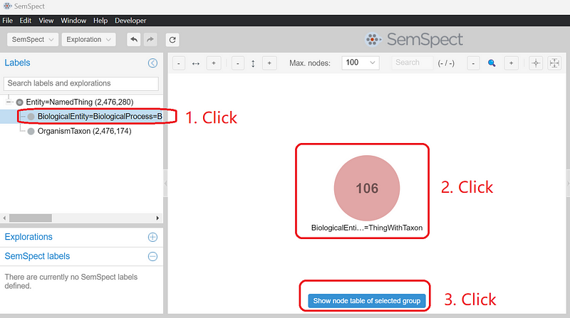
Let’s investigate how the nitrate reduction pathway is distributed among bacteria. Click the BiologicalEntity… label under Labels. On the main canvas, a circle appears. The number 106 indicates that there are a total of 106 biological process nodes in the graph. Click the circle and then click the blue button Show node table of selected group (Figure 6).

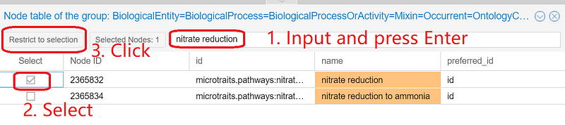
In the node table, enter “nitrate reduction” and press “Enter”. Select “nitrate reduction” and click “Restrict to selection” (Figure 7).

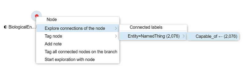
And the circle on the canvas will be reduced to just one node: nitrate reduction. Right-click the small circle and select “Explore connections of the node” ➡️ “Entity=NamedThing (2,076)” ➡️ “Capable_of (2,076)”.

Afterward, a new circle that represents the 2,076 nitrate-reducing taxa appears on the canvas. Select that new circle and click the blue button Show node table of selected group to open the taxon table. There, you can see all the taxa.

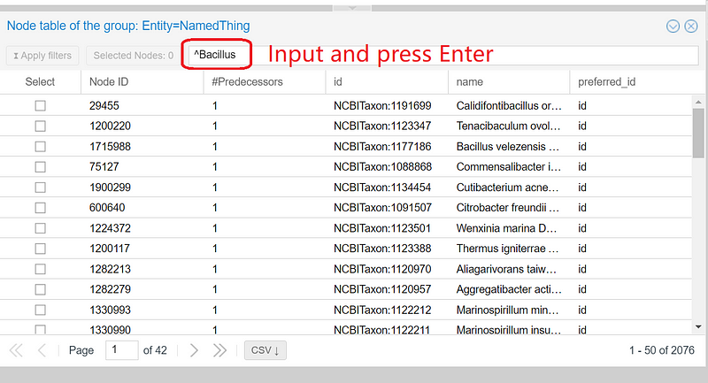
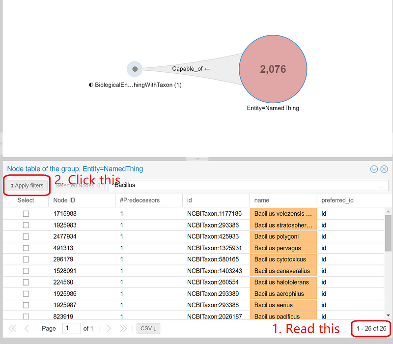
In SemSpect, we can use regular expressions to filter the results. For example, if we want to know how many bacteria are from the genus Bacillus, we can enter “^Bacillus” or “^bacillus[\s_]” in the input field and press enter. SemSpect quickly shows the 26 nitrate-reducing Bacillus in the dataset. Click “Apply filters” to narrow the “NamedThing” circle down to the 26 Bacillus, which are represented by 26 small dots inside the circle (the central big red circle in Figure 10).

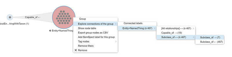
We can explore these Bacillus further. Right-click the “NamedThing” circle and select “Explore connects of the group” ➡️ “Entity=NamedThing (≥ 467)” ➡️ “Subclass_of <-> (≥ 467)” ➡️ “Subclass_of -> (7)”. This action chain creates a third circle with seven small dots (Figure 11). In other words, the 26 nitrate-reducing Bacillus belong to seven Bacillus subgroups, such as the Bacillus cereus group and the Bacillus subtilis group.

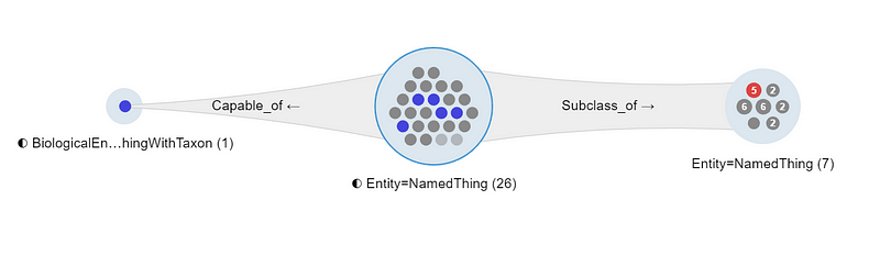
You can even highlight the individual subgroup and its members by clicking the small dots (Figure 11). This gives you a quick sense of how large each subgroup is. Last but not least, you can export these filtered results as a CSV file for further processing.

Conclusion

This article demonstrates how to build a Biolink-compatible knowledge graph with BioCypher and then analyze its content with SemSpect. BioCypher takes over the tedious ontology work and simplifies the import process considerably. The end result is a Biolink-compatible graph, which is easy to share. Perhaps in the future, we can even extend the Biolink model to enable Bayesian inference in knowledge graphs. And domain experts can create their own knowledge graphs and push them onto the knowledge graph hub, just like DockerHub for Docker images. So other bioinformaticians can download, merge and modify those graphs. Such a collaboration mode will without doubt accelerate the adoption of knowledge graphs in biomedical research.

With SemSpect, we quickly got the list of nitrate-reducing Bacillus without a single line of code. SemSpect is also a great data processor because you can export the results for downstream analyses. The interface is intuitive and the execution is fast. Because graph databases can be intimidating at first with their complexity, no-code graph solutions, such as SemSpect and Gemini Cloud, can give non-programmers an easy entry into the field and encourage them to learn more.

This article only touches the surface of the two, though. For example, BioCypher can reify relations as nodes instead of edges. As a result, we can add information source nodes to the relations. BioCypher can write data into Neo4j directly in the “online” mode, although I cannot make that work on my computer. You can learn their other features in the tutorials. And I encourage you to build your own Biolink-compatible graphs in your projects.