I Built the Same Virus Knowledge Graph on Gemini Cloud, AuraDB and Neo4j Desktop

No-code vs. Low-code vs. Code; Cloud vs. On-prem

You will learn:

1. how to use the no-code Gemini Cloud to construct a virus knowledge graph

2. to construct the same knowledge graph on Neo4j Desktop and AuraDB

3. some fun facts about influenza, COVID-19, monkeypox, and the common cold

4. the pros and cons

Recently, knowledge graphs are gaining traction quickly. Big tech companies are using them frequently, such as Google’s Infobox, Amazon Music, and Microsoft Academic Knowledge Graph. That should not be a surprise because graphs are excellent at managing knowledge. They store information like a human, that is, via subject-verb-object triples. We can transform many existing data into knowledge graphs and then learn a lot by exploring, searching, and analyzing them.

The construction is straightforward: we break down our domain knowledge into a series of subject-verb-object triples and write them into a collection of CSV files. We then import them into a graph database, such as Neo4j. Voilà! And you can see how I built my knowledge graph for the Carbohydrate-Active enZYmes (CAZy) in this article.

During data preparation, we need to pay extra attention to the data quality so that the graph represents our knowledge fully. This step usually took the most time. But the steps that follow are important, too. Because there can be many CSV files that represent many types of nodes and relations in a given project, a good data importer can ease the process considerably. After the import, a good GUI can help us explore the content and discover new insights. Finally, it would be nice if the graph platform has integrated statistics or even machine learning in its interface.

Neo4j has always been my graph database of choice. Its query language Cypher is easy to learn and write. The database is powerful and fast. Neo4j has powered my medical chatbot Doctor.ai (1, 2, 3, 4, 5, 6, 7, and 8). On-prem, we can use Neo4j Desktop to prototype. On the cloud, we can either deploy Neo4j on an EC2, or simply use Neo4j’s own fully-managed AuraDB. No matter which one you choose, some basic Cypher is required. That could be a speed bump for some knowledge graph newbies. So for people who want to dive headfirst into the knowledge graph, is there any no-code alternative?

Fortunately, the answer is a yes. A startup called Gemini Data from San Francisco has debuted Gemini Explore and its online platform Gemini Cloud in GraphConnect 2022. It is an end-to-end no-code, cloud-native graph database application. Users can import, explore and search the graph data just by clicking and typing. They can also bring their own Neo4j or AuraDB databases to Gemini. Its interface is similar to Neo4j Bloom, but it comes with the much-needed aggregate functions. So Neo4j users should feel quite at home with Gemini Cloud. In the future release, Gemini will be able to do semantic searches, like Doctor.ai or Ask Data from Tableau. And it will also be able to connect to our local graph databases. Under the hood, Gemini stores the user graph data either in Neo4j (default), TigerGraph, Dgraph, ArangoDB, JanusGraph or AWS Neptune. Currently, the Gemini Cloud is in closed beta. And it will be available in August 2022. And a guided tour will also be available by then.

Gemini Data has kindly provided me with a trial version. It came at the right time because I needed to build a new knowledge graph about the viruses myself. So I made it with Gemini Cloud, Neo4j Desktop, and AuraDB. In this article, I want to document the processes and explain their pros and cons. And we are going to learn something interesting about influenza, COVID-19, monkeypox, and the common cold along the way. The data and scripts for this project are hosted on my GitHub repository here.

1. Data preparation

The data comes from two sources: the Kyoto Encyclopedia of Genes and Genomes (KEGG) and the Virus-Host Database (VHDB). On the one hand, the KEGG database has kept a comprehensive list of viruses, their proteins, and drugs that target them. On the other hand, the VHDB complements KEGG with detailed information about the viral hosts and diseases. Because VHDB has normalized its data entities with the KEGG identifiers, it was quite easy to link the two data sources together. I have downloaded the database in TSV format from VHDB. Then I used KEGG’s REST API to download all the information for my knowledge graph. Finally, I formatted them into CSV.

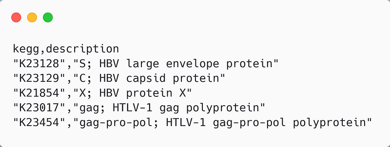
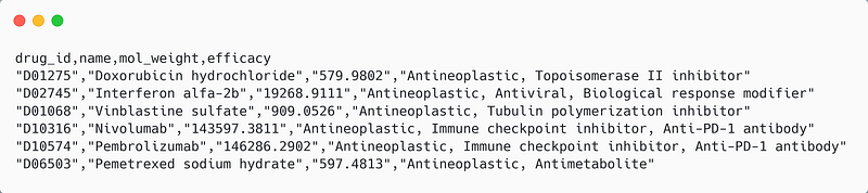
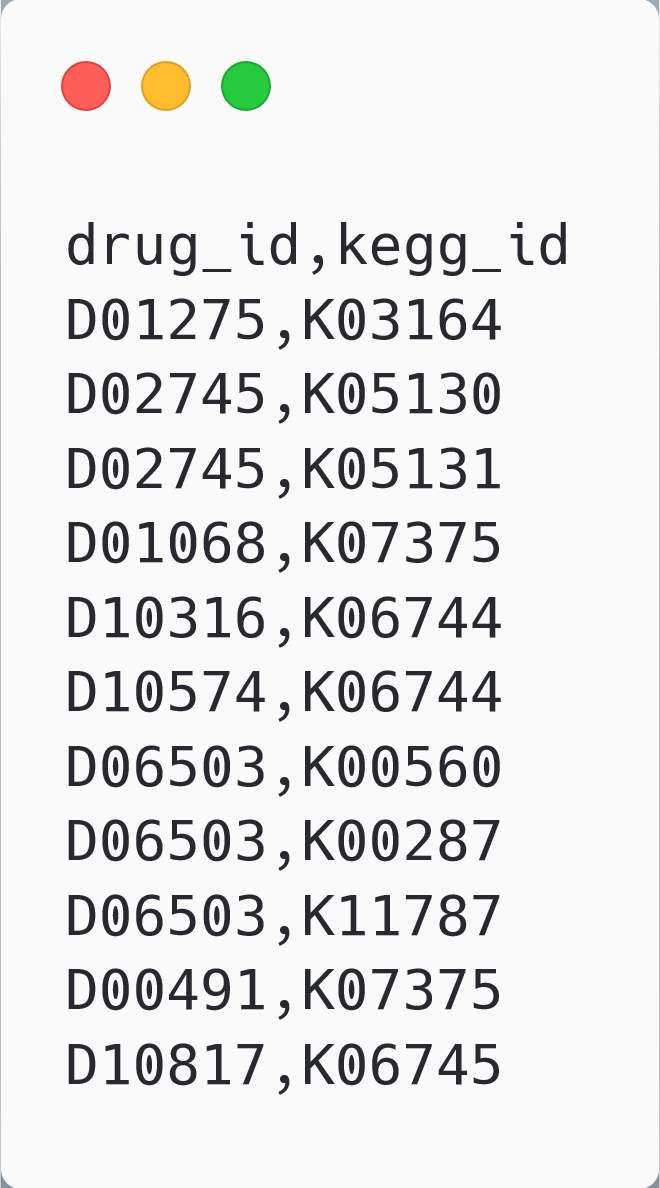
Because the same data will be imported into three platforms, I separate the data into two types of files: node and relation. The node files contain an ID column and other property fields. They define the nodes. And the relation files connect the nodes using their IDs. They look like so.

2. Import in Gemini Cloud

The free Gemini only supports CSV import, while the paid version will support many other data sources and types. Once the data were ready, I logged into my Gemini console and created a new project called virus_kg. I clicked the Data Modeling button and afterward the + Create Flow button to begin the first data import.

Gemini Cloud breaks down the data modeling process into subprocesses called flows. In each flow, we just work with one CSV file (Figure 3). It turns out that the import order is also important because the late imports overwrite the early ones. After examining my data, Gemini taught me to import the relation files before the node files. So I began with the host_taxon_connections.csv file like this (Figure 3).

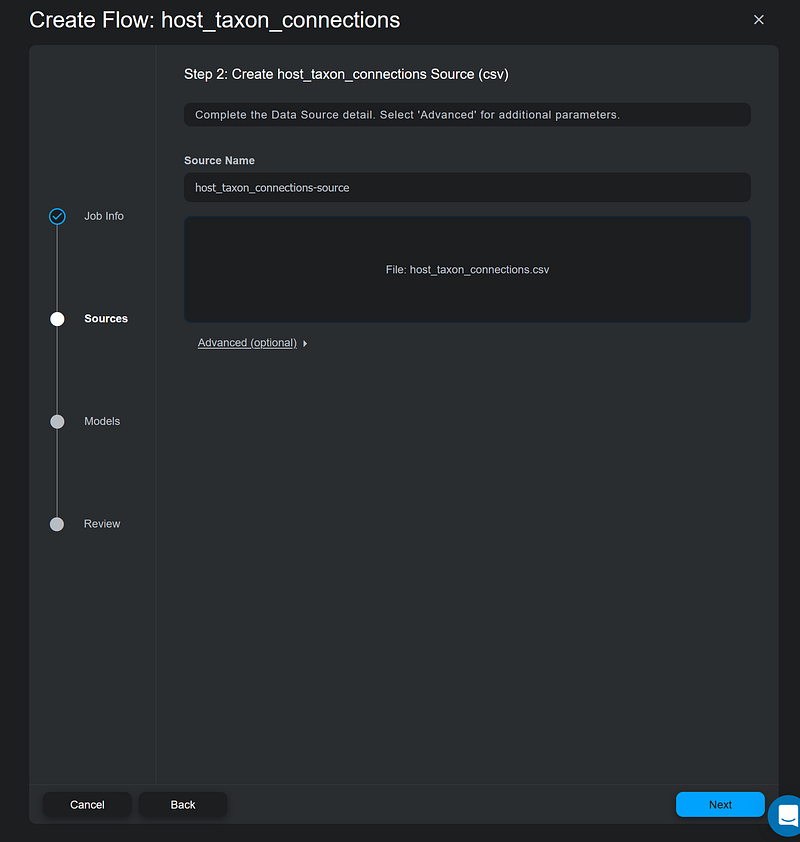
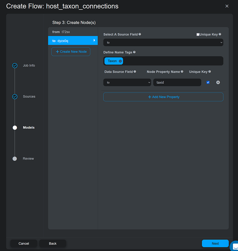
This file establishes the taxonomic hierarchy in my knowledge graph. Taxonomy organizes organisms with shared characteristics together as a taxonomic group and assigns the group to a taxonomic rank. This group can be merged with other relative groups to form a more inclusive one of higher rank. The host_taxon_connections.csv contains two columns: from and to. In each line, the from column is the taxon to which the to column taxon belongs. I filled both columns with the NCBI taxids. In Step 3, I created two Taxon nodes for both columns. I also set the taxid as their node property names. For Neo4j users, Name Tag is Gemini’s way of saying node label. According to Gemini, I needed to remove the check mark next to Unique Key but activate the one next to taxid (Figure 4).

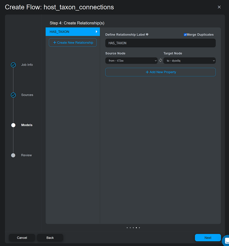
Next, I defined the HAS_TAXON relation between the from and the to nodes (Figure 5).

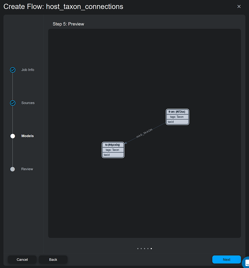
Then it came to the Preview page. It visualized how the nodes and the relation appear in the graph (Figure 6).

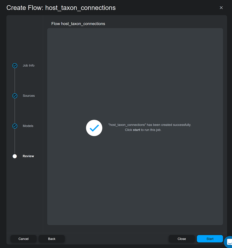
On the Review page, I simply clicked Close instead of Start. So I could run all the flows later in the overview stage. It gave me the chance to modify the flows in case of misconfiguration.

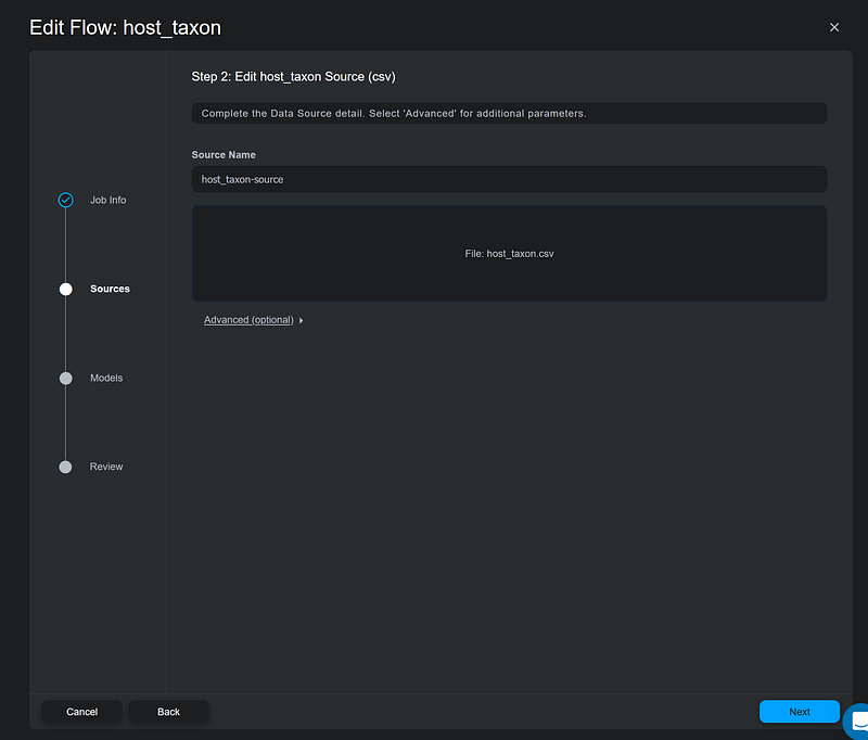
After configuring the host_taxon_connections flow, I worked with the host taxon nodes. I created a new flow with the host_taxon.csv as its source (Figure 8).

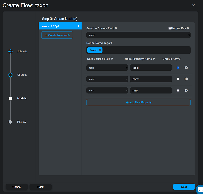
On the Create Node(s) page, Gemini taught me to enter the property that I would like to display later in the knowledge graph under the Select A Source Field field. For the Taxon node, that property would be name. Again, I set Taxon as the node label. And I also added all the properties, such as taxid, name, and rank from the CSV file to the node. Here, I also unchecked Unique Key next to the Select A Source Field, but checked the one next to the taxid (Figure 9).

Since it was a node importing flow, there was no need to define any relation in it. After the configurations of the host_taxon_connections.csv and host_taxon.csv, I simply repeated the process and imported all the files (Figure 10).

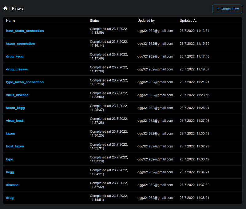
The overview page also allows me to review and run the flows. If any of the flow fails, I can click into that flow, go through the wizard pages, and fix the error.

3. Data exploration in Gemini Cloud

3.1 Influenza

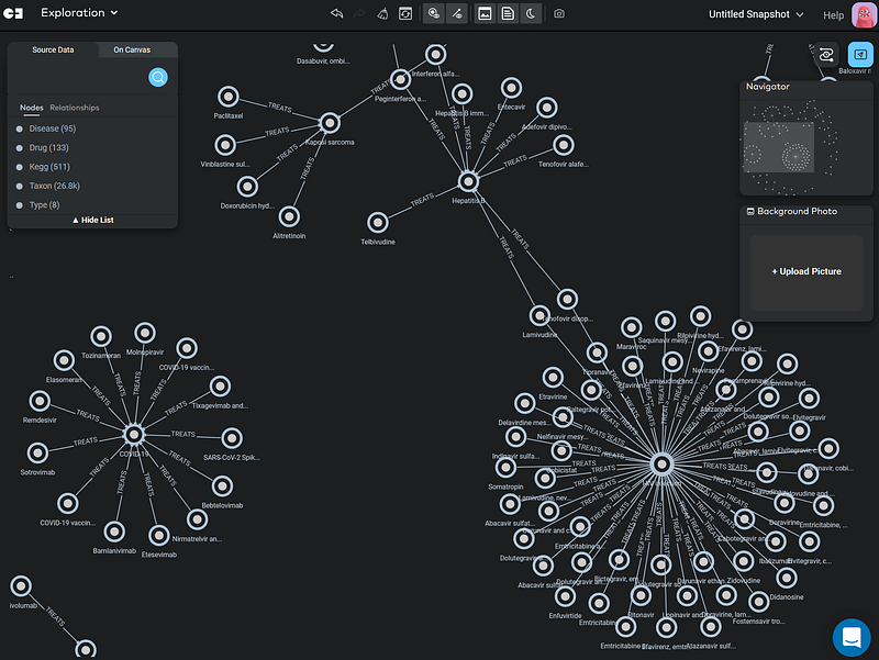
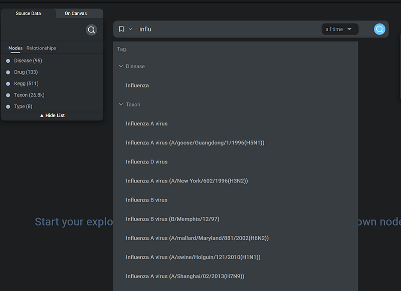
After the import, I went to Gemini’s Explore Nodes/Exploration mode to browse the knowledge graph. In the following figure, you can see that as I typed influ, the search bar immediately suggested the Disease node in its dropdown (Figure 11).

Then Gemini Cloud executed the search and the Influenza node appeared on the canvas. When I left-clicked the node, I could read the node properties, such as its description and category. Next, I right-clicked the node to open the context menu in order to explore its neighbors (Figure 12).

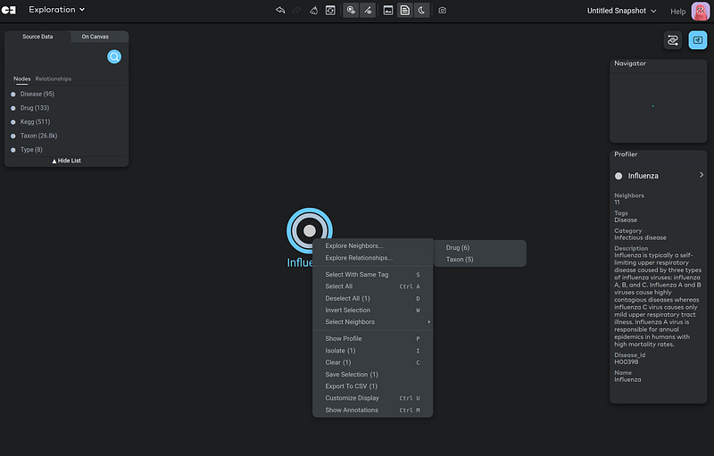
Gemini Cloud showed two types of nodes connected to this Influenza node: Drug (6 nodes) and Taxon (5 nodes) (Figure 12). Here, I chose the drug nodes (Figure 13).

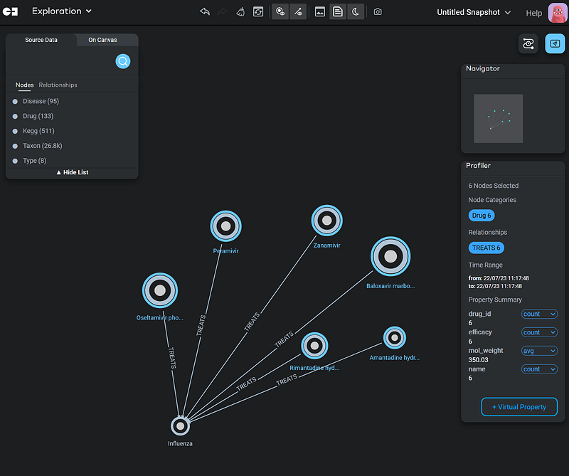
Gemini Cloud allows me to select a group of nodes and calculate some statistics easily. Here, I calculated the average molecular weight of the six drugs just by selecting them and choosing avg in the drop-down on the Profiler panel.

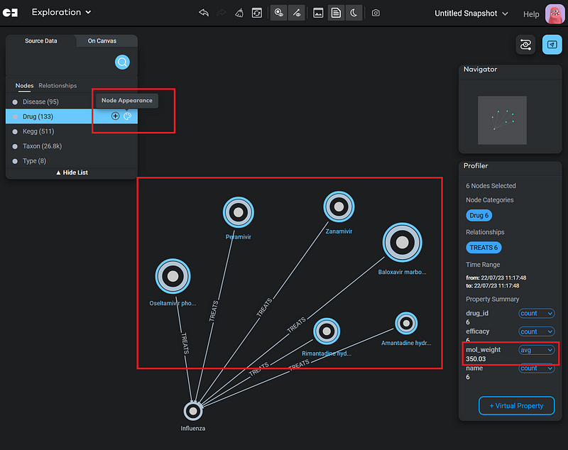
Gemini allows us to do both conditional display and conditional search based on node properties. For example, I scaled the node size according to the molecular weight in Figure 14. The higher the molecular weight, the larger the node. This is called conditional display. And it can be set up in Node Appearance (the color palette icon).

3.2 COVID-19

Next, I clicked the TARGETS relation and opened 200 nodes/relations in the graph. The TARGETS relations connect drugs and their viral target proteins (Kegg). It was not hard to find the COVID-19 cluster.

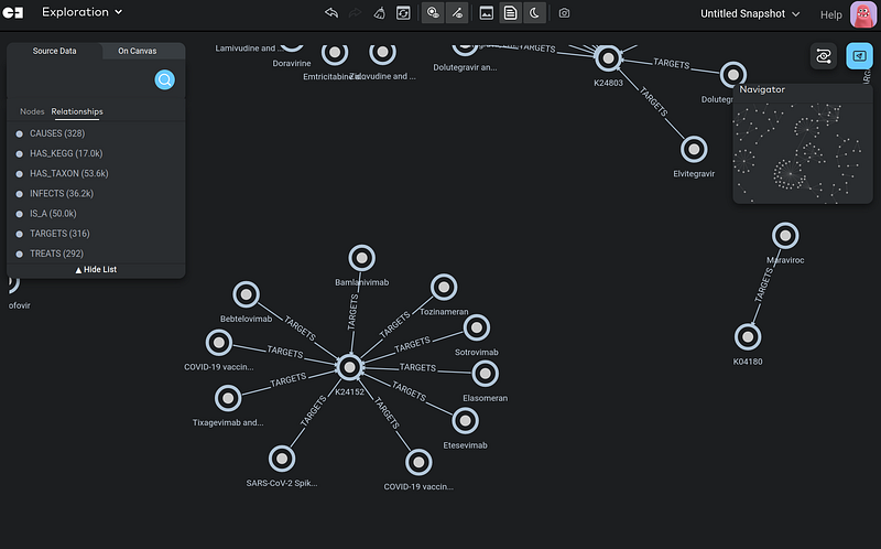
Then I expanded K24152‘s neighbors a bit, select all the nodes, and clicked Isolate in the context menu. As a result, Gemini removed all the other nodes except this cluster.

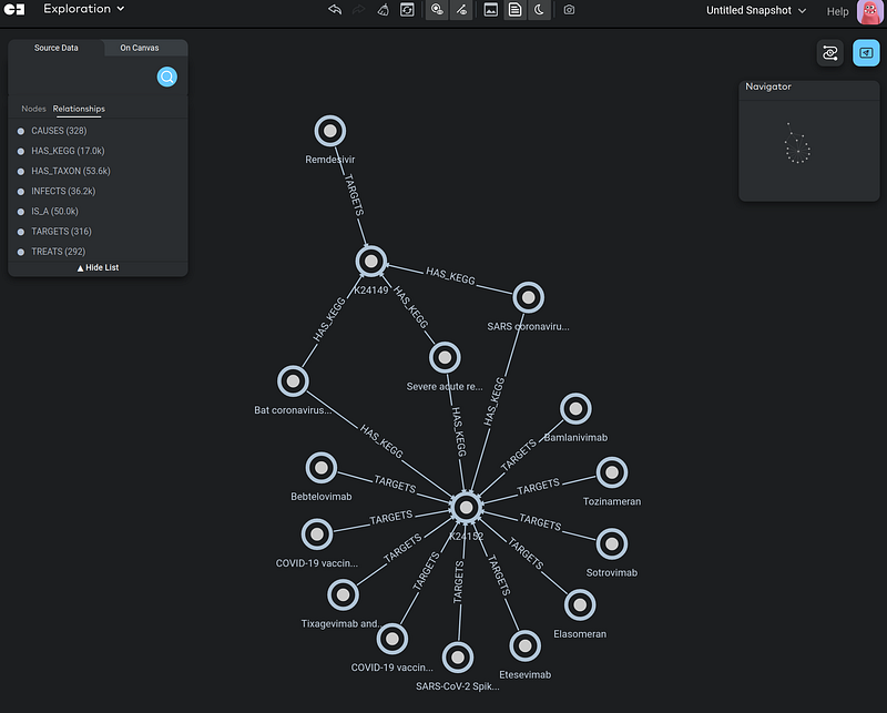
This little research immediately made it clear that the vaccines and Remdesivir act on different parts of the coronaviruses. We can see that SARS, SARS-CoV2 (the pathogen behind COVID-19), as well as the Bat coronavirus all have the spike glycoprotein (S) and replicase polyprotein. The spike protein is targeted by a number of vaccines, while the replicase is targeted by Remdesivir.

I played a bit more with my knowledge graph in Gemini Cloud. And I am still impressed by its feature-rich interface and context menus. The graph rendering was fast and responsive. And it provides us with lots of control over the visualizations, too.

4. Import in Neo4j Desktop

Next, I imported the same data into my Neo4j Desktop on my local computer. The CSV files were first transferred to the project’s import folder and then imported into the database with the following commands. Please read “1. Import the data into Neo4j” from this article if you need more details.

5. Import in AuraDB

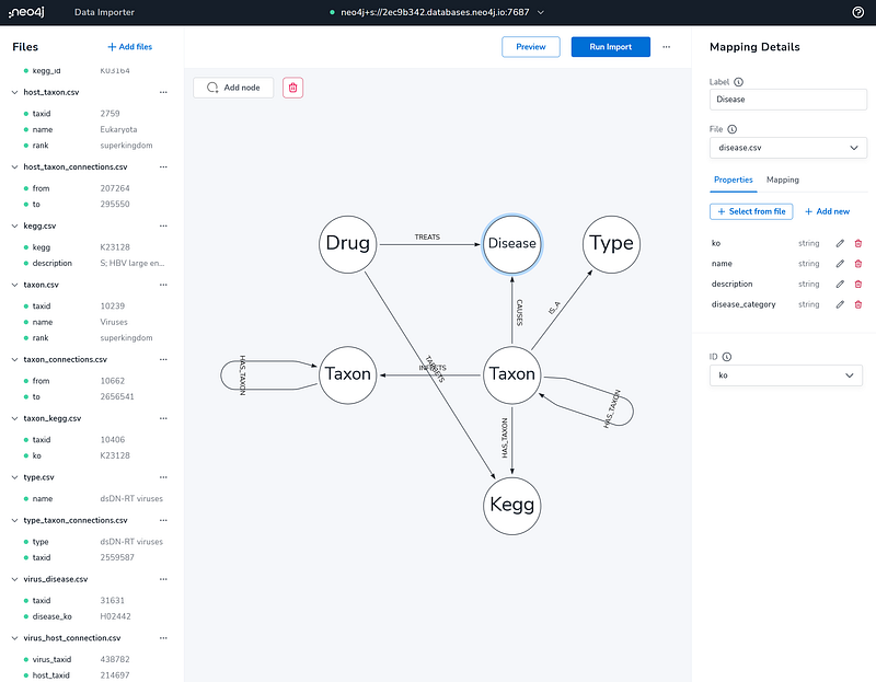
The cloud platform AuraDB from Neo4j has its own Data Importer. I dragged and dropped all the CSV files into its Files panel. On the central canvas, I drew the nodes and their relations. On the right panel, I defined their labels and properties. If you need more details, please read “3. Create a Neo4j project in Aura and import data” in my previous article.

6. Data exploration in Neo4j Desktop and AuraDB

Both the Neo4j Browser and Bloom work the same way in the Desktop and AuraDB. Here, I show some of my data explorations in AuraDB.

6.1 Monkeypox

Currently, we are watching a monkeypox outbreak anxiously in many parts of the world. Let’s check it out in my knowledge graph. Because the monkeypox virus belongs to the genus Orthopoxvirus, I examined the latter and its neighbors with this Cypher.

The command returned the following network.

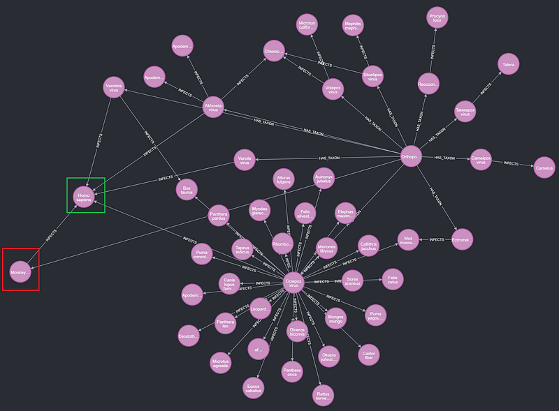
We can immediately see that the monkeypox virus (red rectangle in Figure 18) is not the only pathogen under Orthopoxvirus that can infect the human population (green rectangle in Figure 18). The others are Variola virus, Vaccinia virus, Cowpox virus, and Akhmeta virus. Among them, Variola viruses cause smallpox. The Cowpox virus is the pathogen of cowpox, which is much milder than smallpox. People observed that dairy farmers who got cowpox were then immune to smallpox. And that was the beginning of the modern smallpox vaccine. The word vaccination comes from the Latin word vaccinus, and it means “of or from the cow”. However, the most recent third-generation smallpox vaccine was no longer from the cow. It comes from attenuated Vaccinia strains instead. Finally, the Akhmeta virus was discovered in July 2013 in Akhmeta, Georgia.

6.2 The common cold

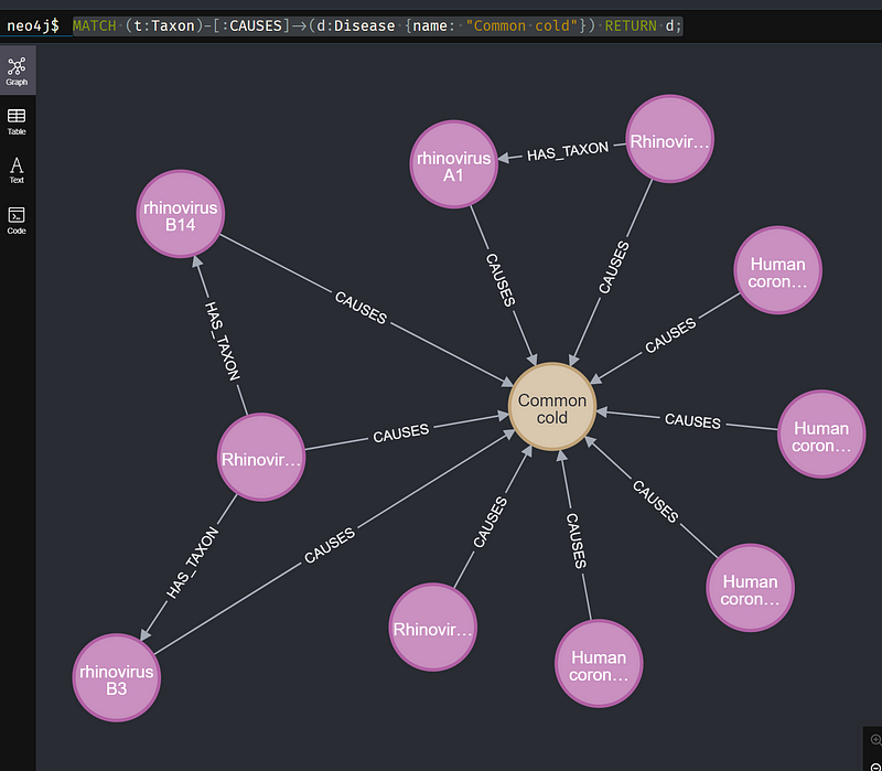
Now let’s check out the common cold and its causative pathogens with the following Cypher.

On hearing “coronavirus”, we now universally think about the Middle East respiratory syndrome-related coronavirus (MERS-CoV, which also appeared in the first episode of the Japanese drama Unnatural), SARS-CoV-1 (pathogen of the SARS pandemic between 2002–2004), and SARS-CoV-2 (pathogen of COVID-19). But the query above revealed that these three headline grabbers have four siblings: HCoV-NL63, HCoV-OC43, HCoV-HKU1, and HCoV-229E. And these four just cause the mild common cold, which is the most frequent infectious disease in humans.

6.3 Graph algorithms

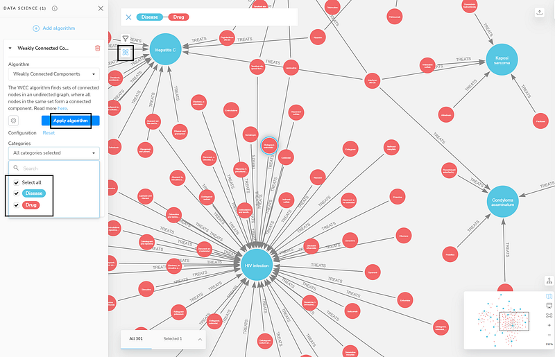
Finally, Neo4j Bloom has integrated some graph machine learning in its interface. To use it, I first installed and activated the Graph Data Science (GDS) plugin on the Neo4j project page. Here, I wanted to see which diseases are connected via common drugs. So I used the Weakly Connected Components algorithm to cluster the Disease and Drug nodes in Bloom.

In the search bar, I first clicked the Disease label. Then Bloom suggested the search phrase Disease-Drug. Once the search was confirmed, Bloom returned a Disease-Drug network. Then I clicked the Show Data science button (the little atom) to open the Data Science panel. I chose the Weakly Connected Components algorithm from the drop-down. I also selected all the categories before I clicked the Apply algorithm button (Figure 20).

It just took a second for the algorithm to run. Afterward, I activated the Rule-based styling to see the clusters.

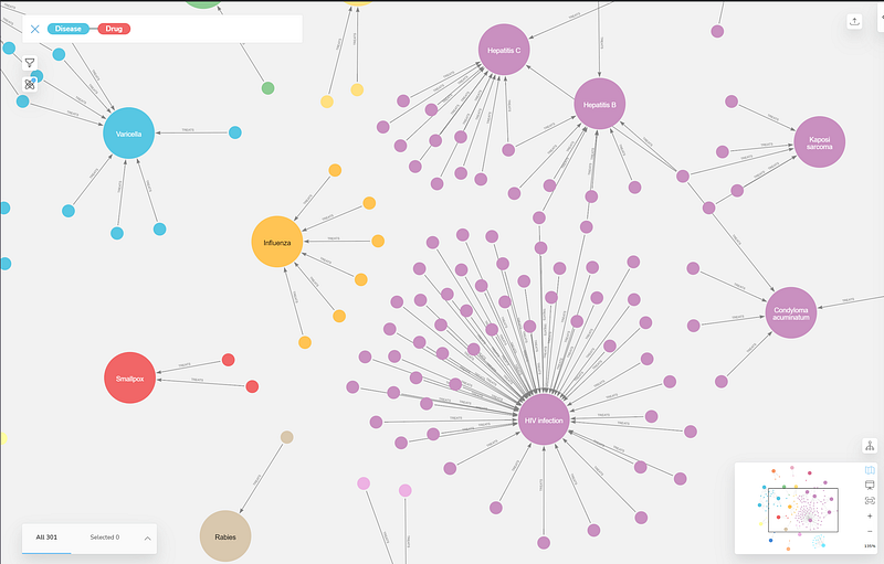
As you can see, HIV infection, Hepatitis B and C, condyloma acuminatum (caused by human papillomavirus (HPV)), respiratory syncytial virus infection, and kaposi sarcoma have formed a large cluster. Interferon alfa-2b, in particular, has connected four of these Disease nodes. It is an antiviral or antineoplastic drug. And it is used for a wide range of indications, including viral infections and cancers.

Conclusion

In this project, I have constructed a virus knowledge graph on three platforms: Gemini Cloud, Neo4j Desktop, and AuraDB. They are all great tools. Gemini’s end-to-end no-code approach can give new users a head start into graphs, while experienced users may enjoy more control in Neo4j Desktop and Bloom. And my summary is as follows.

Gemini Cloud and Neo4j’s own AuraDB are both in the cloud. So it is a great way to share your work with your friends. Also, we don’t need to worry about the infrastructure because the providers manage it for us. However, I think it is a good idea to prototype your knowledge graph first on the Neo4j Desktop before you move to the cloud. In that case, you can catch and fix the data bugs locally.

Both AuraDB and Gemini Cloud provide us with no-code data importers. But compared to AuraDB’s, the import utility in Gemini takes some getting used to. I needed to create a dozen of flows to import all the files. And I had to click and type through several wizard pages to set things up in each flow. For a large collection of files, that was error-prone. Unfortunately, Gemini Cloud’s current version does not allow any data editing. As a result, even one tiny mistake, as insignificant as a typo in the node label, can ruin the whole batch. In that case, I had to purge the project, click through every single one of those wizard pages, correct the error, and start the flow again. Furthermore, Gemini’s interface needs some polishing. For example, the Unique Key checkboxes are confusing. Also, the “name tag” concept needs clarification. For Neo4j users, it is basically a node label.

In comparison, AuraDB’s Data Importer is very neat, visual, and intuitive. The bottom line is that it cost me far less time than Gemini’s flows. I could easily complete the import without any help. On the local front, we still have to use Cypher to import CSV in Neo4j Desktop. It would be really cool if Neo4j could bring AuraDB’s Data Importer to the Desktop.

The next battlefield is analytics. Gemini Cloud has done a great job. It has forgone the iterative update strategy in its network visualization. This strategy updates the node positions constantly and is computationally very expensive. As a result, the interface is more responsive. And I didn’t need to keep track of all those moving nodes. To update the layout, I simply clicked the Redraw Graph button. And its search was intelligent and fast. In contrast, the full-text search in Neo4j Bloom does not seem functional at all. Gemini’s no-code aggregation function is also a much-welcomed addition. I didn’t even know that I needed this feature before, but now I cannot live without it. The conditional display and conditional search are also very useful.

The Gemini team told me that users can access the graph database via the Neo4j driver in the future. So at the moment, Gemini Cloud cannot act as a backend yet. Right now, Gemini can highlight the shortest path between two nodes. But if you want to do more advanced graph data science, Neo4j is still your only choice. The Gemini team are catching up though by adding more machine learning algorithms in different parts of their product. Finally, users can write Cypher in Neo4j Explorer or Bloom to do complex searches. But that is not possible in Gemini.

Graph databases are trending. So we need simple but powerful tools to make the most out of them. Just like what Tableau has done for data science, Gemini and Neo4j have made interactions with graph databases much easier. These products are still evolving. Gemini will have a dashboard and NLP search functionalities in the future release. Gemini can learn how to import and edit data, do graph machine learning, and act as a backend from Neo4j, while Neo4j can learn how to do statistics in the GUI from Gemini. Or they can join forces. In any case, the users benefit.

I thank Gemini Data for their support in this article.

Academic users may freely use the KEGG website. Virus-Host DB is licensed under a Creative Commons Attribution-NonCommercial-ShareAlike 4.0 International License.