Machine Learning Project 14 — Naive Bayes Classifier — Step by Step

If you are like me and enjoy Mathematics, then you’ll definitely enjoy this article. Before getting into the Naive Bayes Classifier, let’s look at the Bayes Theorem.

#100DaysOfMLCode #100ProjectsInML

Bayes Theorem

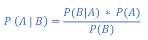
To understand the Bayes theorem, let’s walk through a simple probability example.

Let’s say we have 2 factories Factory 1 and Factory 2 manufacturing laptops. The laptops are labelled so we know which laptop came from which factory. During the testing phase, we find some defective laptops.

This is the information that is given to us.

1. Factory 1 produces 30 laptops per hour.
2. Factory 2 produces 20 laptops per hour.
3. 1% of all laptops are defective.
4. 50% of defective laptops came from Factory 1.
5. 50% of defective laptops came from Factory 2.

What is the probability that a laptop manufactured by Factory 2 is defective?

A question like this can be answered using Bayes Theorem.

Let’s write the above 4 points in Mathematical terms or in terms of Probability.

We know from above points (1, 2) , that Factory 1 produces 30 laptops/hour and Factory 2 produces 20 laptops/hour — so in a given hour a total of 50 laptops are produced.

Factory 1 produces 30 laptops per hour — The probability of the laptop coming from Factory 1 — meaning the probability that any laptop that we pick up from the 50 laptops has come from Factory 1 is:

P(Factory 1) = 30/50 = 0.6 or 60%

Factory 2 produces 20 laptops per hour — Similarly the probability of the laptop coming from Factory 2 — meaning the probability that any laptop we pick from the 50 laptops has come from Factory 2 is:

P(Factory 2) = 20/50 = 0.4 or 40%

1% of all laptops are defective — Probability of a laptop being defective — meaning of all the laptops produced — 1% are defective.

P(Defective) = 0.01 or 1%

50% of defective laptops came from Factory 1 — This means, if we take only the defective laptops and pick any one from the lot, there is a 50% chance it came from Factory 1.

The way to write that Mathematically is:

P(Factory 1 | Defective) = 0.5 or 50%

The vertical line means “given some condition”. So the way to read this is — the probability of laptop coming from Factory 1 given the condition that it is defective is 50%.

50% of defective laptops came from Factory 2— This means, if we take only the defective laptops and pick any one from the lot, there is a 50% chance it came from Factory 2.

The way to write that Mathematically is:

P(Factory 2 | Defective) = 0.5 or 50%

The way to read this is — the probability of laptop coming from Factory 2 given the condition that it is defective is 50%.

Our original question is — What is the probability that a laptop manufactured by Factory 2 is defective?

The way to write this Mathematically is

P(Defective | Factory 2) = ???

The condition given is — that the laptop is manufactured by Factory 2. What we need to find is — what is the probability that it is defective?

Now let’s rewrite the Bayes theorem for this problem. Instead of variables A and B — let’s replace with terms used in this problem to get a better understanding.

We have already solved the right hand side of the equation above — so let’s just plug in the values

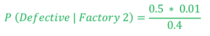
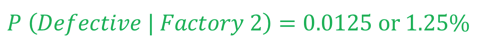
So according to Bayes theorem, the probability that a laptop manufactured by Factory 2 being defective is 1.25%.

How can Bayes theorem be applied to Machine Learning Problem?

I’m assuming the question on everybody’s mind is — how does this apply to Machine Learning classification problem.

If you think about it intuitively, it does right — you are trying to predict something given some conditions right. For example, you might want to predict salary given a person’s age and experience.

Let’s walk through an example and see how we can apply Bayes theorem to a machine learning problem. I’ve taken this example from the A-Z Machine Learning course on Udemy.

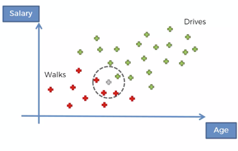
Take a look at the observations in the graph below:

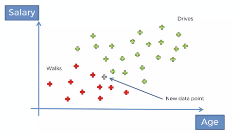
• X axis represents the age of a person
• y axis represent the salary of the person
• The red observation points represent the people who walk to work
• The green points represent the people who drive to work

Now we have a new data point as shown. How do we classify this point. Does this person walk or drive to work?

This is a typical classification problem. Let’s see how we can apply Naive Bayes theorem to solve this machine learning problem.

These are the 3 steps:

1. First, we are going to apply the Naive Bayes theorem to find the probability that this person walks to work given his features*
2. Next, we will apply the theorem again to find the probability that this person drives to work given his features*
3. Then compare the 2 probabilities and see which is greater and assign the new data point to that class.

* What do I mean by features — in the above example, the age and salary of the person represent the features. In reality, the person can have many features but for simplicity we are taking only 2 features.

First Step — Find probability that person walks to work given his features

The diagram below shows the theorem for this problem and the terminology used for each part of the equation.

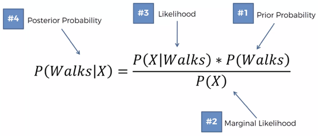
• Calculate Prior Probability — P(Walks) — This is simply the probability that a person walks to work.

P(Walks) =  (Number of people who walk) / Total observations
P(Walks) = 10/30

• Calculate Marginal Likelihood — P(X)

The way we do this is by drawing a circle around our new data point. The radius of that circle is decided by us and is given as an input to the algorithm. As you can see, we have drawn a circle that contains 4 observations along with the new observation. All the points inside the circle are considered to be similar in features to the new observation.

For example if new point has features (Age:25 and Salary $25,000) — we will draw a circle with radius such that anyone between age 20 and 30 and who makes salary between $20k to $30k will be considered similar to the new data point.

So P(X) is the probability that any new data point that we add will fall inside this circle. It is calculated as follows:

P(X) = (Number of Similar Observations) / (Total Observations)
P(X) = 4/30

Number of similar observations is 4 — as we can see there are 3 red points and 1 green point in the circle that we have drawn.

• Calculate the Likelihood — P(X|Walks)

P(X|Walks) specifies — what is the probability that somebody who walks exhibits features X.

P(X|Walks) = (# of observations among ppl who walk) /(Total walkers)
P(X|Walks) = 3/10

From the circle, we can see that number of red dots (walkers) inside the circle are 3 and total number of walkers are 10.

• Calculate Posterior Probability

So now let’s plug in the values to calculate the probability that the person walks to work given his features

P(Walks|X) = (P(X|Walks) *  P(Walks)) / P(X)
P(Walks|X) = (3/10) * (10/30) / (4/30)
P(Walks|X) = 0.75 or 75%

Second Step — Find probability that person drives to work given his features

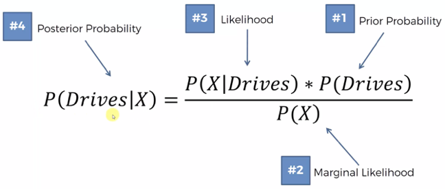
• Calculate Prior Probability — P(Drive) — This is simply the probability that a person drives to work.

P(Drives) =  (Number of people who drive) / Total observations
P(Drives) = 20/30

• Calculate Marginal Likelihood — P(X)

We have already done this above and this value remains the same.

P(X) = (Number of Similar Observations) / (Total Observations)
P(X) = 4/30

• Calculate the Likelihood — P(X|Drives)
• P(X|Drives) specifies — what is the probability that somebody who drives exhibits features X.

P(X|Drives)= (# of observations among ppl who drive)/(Total drivers)
P(X|Drives)= 1/20

From the circle, we can see that number of green dots (drivers) inside the circle are 1 and total number of drivers are 20.

• Calculate Posterior Probability

So now let’s plug in the values to calculate the probability that the person drives to work given his features

P(Drives|X) = (P(X|Drives) *  P(Drives)) / P(X)
P(Drives|X) = (1/20) * (20/30) / (4/30)
P(Drives|X) = 0.25 or 25%

Third Step — Compare the 2 probabilities

P(Walks|X) v.s. P(Drives|X)
0.75 v.s. 0.25
0.75 > 0.25
P(Walks|X) > P(Drives|X)

So it is more likely that this new person with features X is going to walk to work. Hence we will classify the new data point in red as a walker.

Now let’s apply the Naive Bayes classifier to our project.

Project Objective

We will use the same problem that we used in Project 10. We are using the same project and applying different classification algorithms to see which classification model gives the best results.

Let’s see if we get a better accuracy with Naive Bayes classifier compared to Logistic Regression, KNN, SVM with linear kernel and SVM with rbf kernel.

We have a dataset that shows which users have purchased an iPhone. Our goal in this project is to predict if the customer will purchase an iPhone or not given their gender, age and salary.

The sample rows are shown below. The full dataset can be accessed here.

Step 1: Load the dataset

Let’s load the dataset. We have 3 independent variables “Gender” , “Age” and “Salary” and we will assign them to X.

y will contain the dependent variable “Purchased iPhone”.

Step 2: Convert Gender to Number

The Naive Bayes classification algorithm’s cannot handle categorical (text) data. In our data, we have the Gender variable which is in String format. So we have to convert that to numerical format.

We will use the class LabelEncoder to convert Gender to number.

Step 3: Split data into training and test set

For splitting the data into training and testing - We will use 25% of dataset as test sample and 75% as training sample.

Step 4: Feature Scaling

Since the independent variables are of different scale, it’s important to do feature scaling. We will use Standard Scaler for this purpose.

Step 5: Fit Naive Bayes Classifier

We will be using the GaussianNB classifier from the sklearn.naive_bayes library. When we create the object of GaussianNB, it does not take any parameters.

Step 6: Make Predictions

We will call the predict method and pass the test dataset.

Step 7: Evaluate Performance of the Model

You can read in detail about metrics in Project 10.

[[66 2]
 [ 7 25]]
Accuracy score: 0.91
Precision score: 0.9259259259259259
Recall score: 0.78125

We have got 9 (2+7) incorrect predictions and an accuracy score of 91%.

Conclusion

So far we have solved the same problem using Logistic Regression, KNN classifiers, SVM and Kernel SVM. Today we implemented Naive Bayes classifier. Let’s compare the results from all classifiers.

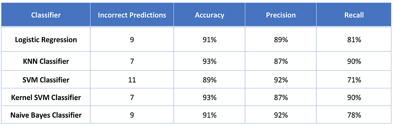
Although the performance is not bad, but still the best results have come from KNN classifier and Kernel SVM classifier.

We have covered 5 classifiers so far. I’ll be covering 2 more in the upcoming articles — Decision Tree and Random Forest classifier.

The full source code can be found here.