LLM Architectures Explained: Encoder-Decoder Architecture (Part 4)

Deep Dive into the architecture & building real-world applications leveraging NLP Models starting from RNN to Transformer.

Posts in this Series

1. NLP Fundamentals
2. Word Embeddings
3. RNNs, LSTMs & GRUs
4. Encoder-Decoder Architecture ( This Post )
5. Attention Mechanism
6. Transformers
7. BERT
8. GPT
9. LLama
10. Mistral

Table of Contents

· 1. Introduction ∘ 1.1 Major Developments in Data Processing · 2. Understanding Sequence Modeling ∘ 2.1 Mastering Sequential Data with Encoder-Decoder Architecture · 3. Encoder-Decoder Architecture ∘ 3.1 The Neural Machine Translation Problem ∘ 3.2 Overview ∘ 3.3 Under the Hood ∘ 3.4 The Encoder Block ∘ 3.4.1 Mathematical Foundations: Encoder ∘ 3.5 The Decoder Block ∘ 3.5.1 Mathematical Foundations: Decoder · 4. Training Encoder-Decoder Models ∘ 4.1 Vectorizing our data ∘ 4.2 Training & Testing of Encoder ∘ 4.3 The Decoder in Training Phase: Teacher Forcing ∘ 4.4 The Decoder in Test Phase ∘ 4.5 The Embedding Layer ∘ 4.6 The Final Visualization at test time · 5. Drawbacks of Encoder-Decoder Models · 6. Improvements in Encoder-Decoder Architecture ∘ 6.1 Adding Embedding Layer ∘ 6.2 Use of Deep LSTMs ∘ 6.3 Reverse the input · 7. Example: Encoder-Decoder Architecture with Neural Networks · 8. Applications of Encoder-Decoder Neural Network Architecture · 9. Sequence-to-Sequence Learning with Neural Networks (Hands-On) ∘ Step 1: Installing and Importing Libraries ∘ Step 2: Data Preprocessing ∘ Step 3: Building the Encoder ∘ Step 4: Building the Decoder ∘ Step 5: Building the Seq2Seq Model ∘ Step 6: Training the Model ∘ Step 7: Evaluate the Model ∘ Step 8: Initialize the Model and Hyperparameters ∘ Step 9: Training Loop ∘ Step 10: Testing with BLEU Score · 10. Conclusion · 11. Test your Knowledge!

1. Introduction

The rapid evolution of Natural Language Processing (NLP) has been marked by significant milestones, none more transformative than the advent of Large Language Models (LLMs). These models have redefined the boundaries of what’s possible in machine understanding and generation of human language. Central to the success of many LLMs is the encoder-decoder architecture, a framework that has enabled breakthroughs in tasks such as machine translation, text summarization, and conversational AI.

The Encoder-Decoder architecture was introduced to address sequence-to-sequence (Seq2Seq) problems, marking a significant breakthrough in handling sequential data.

1.1 Major Developments in Data Processing

1. Tabular Data: Initially, the focus was on utilizing Artificial Neural Networks (ANNs) to process tabular data. This approach evolved into Deep Neural Networks (DNNs) by increasing the number of layers, thereby enhancing the models’ capacity to capture complex patterns within the data.
2. Image Data: In tasks such as object recognition — for instance, identifying whether an image contains a dog or a cat — images serve as 2D grids of data. ANNs are not particularly effective at processing this type of structured data. This limitation led to the development of Convolutional Neural Networks (CNNs), which are specifically designed to interpret and analyze visual information in grid formats.
3. Sequential Data: Sequences like textual or time-series data have meaningful order and temporal dependencies. ANNs and CNNs are not well-suited for handling such data because they lack mechanisms to capture sequential relationships. This gap was filled by Recurrent Neural Networks (RNNs) and their advanced variants, Long Short-Term Memory (LSTM) networks and Gated Recurrent Units (GRUs), which are capable of modeling and learning from temporal patterns.
4. Seq2Seq Data: In certain applications, both the input and output are sequences, as seen in machine translation tasks. Traditional models struggle with this type of data due to the complexities involved in aligning input and output sequences of variable lengths. This challenge necessitated the development of specialized architectures capable of effectively handling Seq2Seq data, paving the way for more sophisticated models in natural language processing.

The focus of this blog is to deal with Seq2Seq Data Problems.

2. Understanding Sequence Modeling

Sequence modeling use cases involve problems where the input, output, or both consist of a sequence of data, such as words or letters.

Consider a very simple problem of predicting whether a movie review is positive or negative. Here our input is a sequence of words and output is a single number between 0 and 1. If we used traditional DNNs, then we would typically have to encode our input text into a vector of fixed length using techniques like BOW, Word2Vec, etc. But note that here the sequence of words is not preserved and hence when we feed our input vector into the model, it has no idea about the order of words and thus it is missing a very important piece of information about the input.

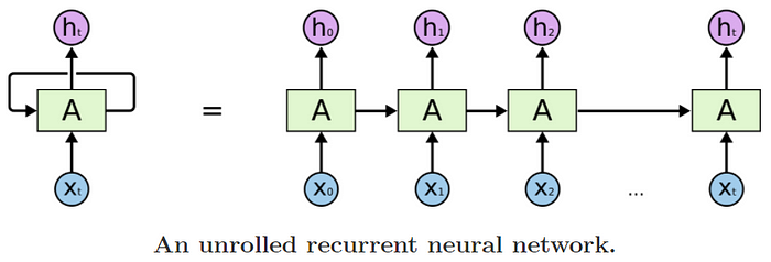
Thus to solve this issue, RNNs came into the picture. In essence, for any input X = (x₀, x₁, x₂, … xₜ) with a variable number of features, at each time-step, an RNN cell takes an item/token xₜ as input and produces an output hₜ while passing some information onto the next time-step. These outputs can be used according to the problem at hand.

The movie review prediction problem is an example of a very basic sequence problem called many-to-one prediction. There are different types of sequence problems for which modified versions of this RNN architecture are used.

Sequence problems can be broadly classified into the following categories:

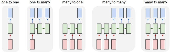
Each rectangle is a vector and arrows represent functions (e.g. matrix multiply). Input vectors are in red, output vectors are in blue and green vectors hold the RNN’s state (more on this soon).

From left to right:

(1) Vanilla mode of processing without RNN, from fixed-sized input to fixed-sized output (e.g. image classification).

(2) Sequence output (e.g. image captioning takes an image and outputs a sentence of words).

(3) Sequence input (e.g. sentiment analysis where a given sentence is classified as expressing positive or negative sentiment).

(4) Sequence input and sequence output (e.g. Machine Translation: an RNN reads a sentence in English and then outputs a sentence in French).

(5) Synced sequence input and output (e.g. video classification where we wish to label each frame of the video).

Notice that in every case are no pre-specified constraints on the lengths sequences because the recurrent transformation (green) is fixed and can be applied as many times as we like.

— Andrej Karpathy, The Unreasonable Effectiveness of Recurrent Neural Networks

2.1 Mastering Sequential Data with Encoder-Decoder Architecture

Sequences are ubiquitous in our world — found in language, speech, financial time series, and genomic data — where the order of elements is crucial. Unlike fixed-size data, sequences present unique challenges in understanding, predicting, and generating information. Traditional Deep Neural Networks (DNNs) perform well on tasks with fixed-dimensional inputs and outputs but struggle with sequence-to-sequence tasks like machine translation, where inputs and outputs vary in length and are unaligned. Therefore, specialized models are needed to effectively handle sequential data.

Research Paper : Sequence to Sequence Learning with Neural Networks

Motivation

The Encoder-Decoder architecture is relatively new and had been adopted as the core technology inside Google’s translate service in late 2016. It forms the basis for advanced sequence-to-sequence models like Attention models, GTP Models, Transformers, and BERT. Hence, understanding it can be very crucial before moving onto advanced mechanisms.

Key Components

• Encoder: The encoder processes the input sequence and encodes the information into a fixed-length context vector (or a sequence of vectors). This encoding captures the essence of the input data, summarizing its informational content.
• Decoder: The decoder takes the context vector provided by the encoder and generates the output sequence, one element at a time. It uses the information from the context vector to produce outputs that are relevant and coherent concerning the input.

3. Encoder-Decoder Architecture

3.1 The Neural Machine Translation Problem

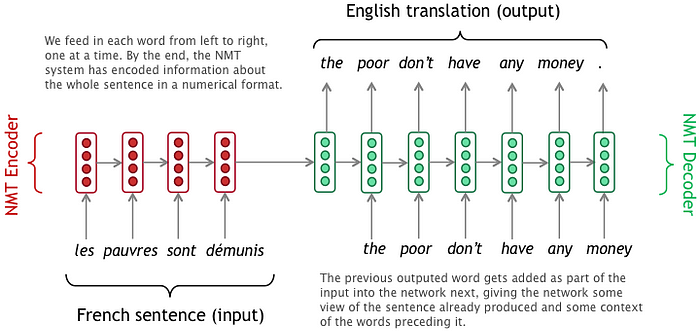
To illustrate this concept, let’s use Neural Machine Translation (NMT) as a running example. In NMT, the input is a sequence of words processed one after another, and the output is a corresponding sequence of words.

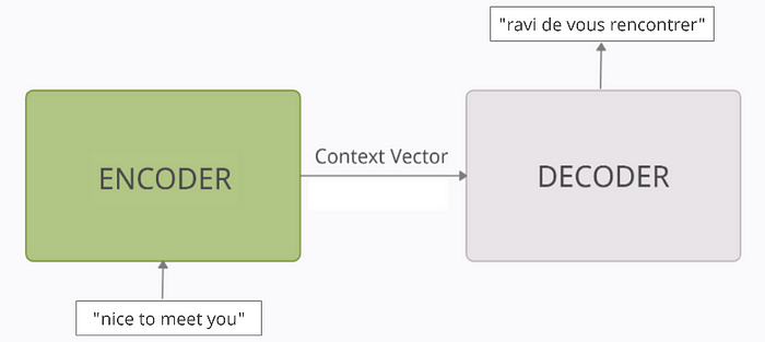
Task: Predict the French translation for an English sentence. Example: Input: English sentence: “nice to meet you” Output: French translation: “ravi de vous rencontrer”

Terms Used: - The input sentence “nice to meet you” will be referred to as X or the input sequence. - The output sentence “ravi de vous rencontrer” is referred to as Y_true or the target sequence, which is the ground truth we want the model to predict. - The model’s predicted sentence is Y_pred, also called the predicted sequence. - Each word in the English and French sentences is referred to as a *token*.

Thus, given the input sequence “nice to meet you”, the goal is for the model to predict the target sequence, Y_true, which is “ravi de vous rencontrer.”

3.2 Overview

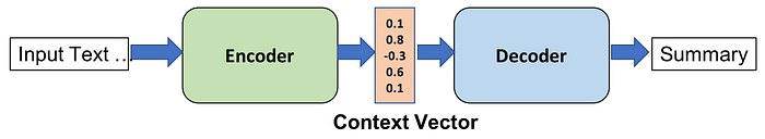
At a very high level, an encoder-decoder model can be thought of as two blocks, the encoder and the decoder connected by a vector which we will refer to as the ‘context vector’.

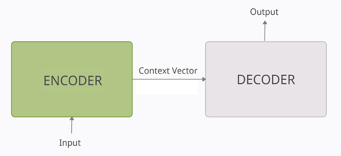
• Encoder: The encoder processes each token in the input-sequence. It tries to cram all the information about the input-sequence into a vector of fixed length i.e. the ‘context vector’. After going through all the tokens, the encoder passes this vector onto the decoder.
• Context vector: The vector is built in such a way that it’s expected to encapsulate the whole meaning of the input-sequence and help the decoder make accurate predictions. We will see later that this is the final internal states of our encoder block.
• Decoder: The decoder reads the context vector and tries to predict the target-sequence token by token.

3.3 Under the Hood

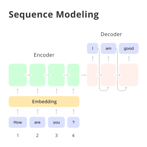
The Seq2Seq model is an RNN-based model designed for tasks such as translation and summarization, where a sequence is taken as input and a sequence is output.

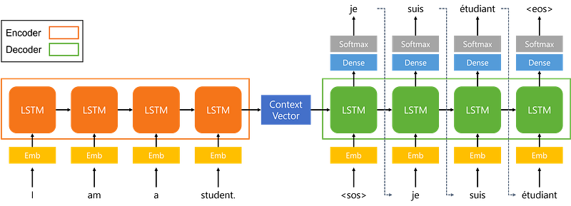
This is a Seq2Seq model that translates the English sentence “I am a student.” to French “Je suis étudiant.” The left orange rectangle represents the encoder, and the right green rectangle represents the decoder. The encoder takes the input sentence (“I am a student.”) and outputs a context vector, while the decoder takes the context vector (and the <sos> token) as input and outputs the sentence ("Je suis étudiant.").

As far as architecture is concerned, it’s quite straightforward. The model can be thought of as two LSTM cells with some connection between them. The main thing here is how we deal with the inputs and the outputs. I will be explaining each part one by one.

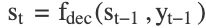
3.4 The Encoder Block

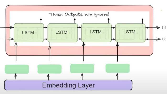
The encoder part is an LSTM cell. It is fed in the input sequence over time and it tries to encapsulate all its information and store it in its final internal states hₜ (hidden state) and cₜ (cell state). The internal states are then passed onto the decoder part, which it will use to try to produce the target sequence. This is the ‘context vector’ that we were earlier referring to.

The outputs at each time step of the encoder part are all discarded

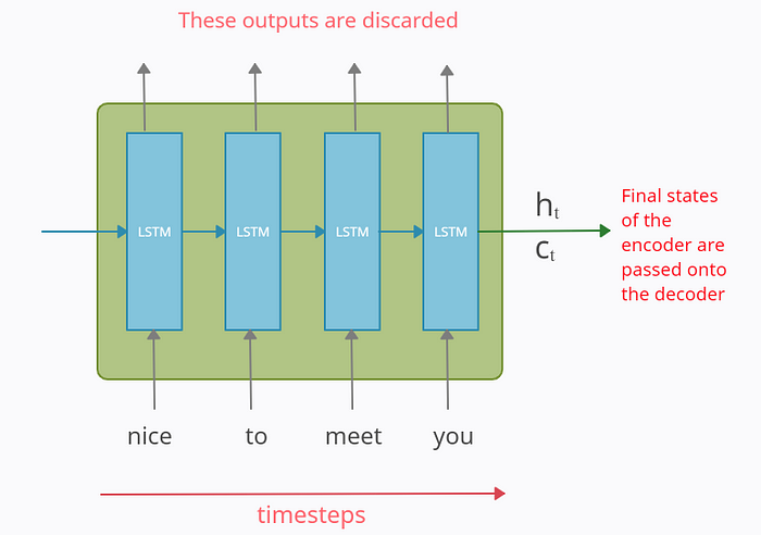
Note: The above diagram is what an LSTM/GRU cell looks like when we unfold it on the time axis. i.e. it is the single LSTM/GRU cell that takes a single word/token at each timestamp.

In the paper, they have used LSTMs instead of classical RNNs because they work better with long-term dependencies.

3.4.1 Mathematical Foundations: Encoder

Given an input sequence:

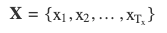
The encoder processes each element sequentially:

1. Initialization: The encoder’s initial hidden state h0​ is typically initialized to zero or learned parameters.
2. Hidden State Updates: For each time step t in the input sequence:

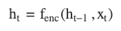
where:

• ht​ is the hidden state at time t.
• fenc​ is the encoder’s activation function (e.g., an LSTM or GRU cell).

3. Context Vector: After processing the entire input sequence, the final hidden state hTx​​ becomes the context vector c:

3.5 The Decoder Block

So after reading the whole input-sequence, the encoder passes the internal states to the decoder and this is where the prediction of output-sequence begins.

The decoder block is also an LSTM cell. The main thing to note here is that the initial states (h₀, c₀) of the decoder are set to the final states (hₜ, cₜ) of the encoder. These act as the ‘context’ vector and help the decoder produce the desired target-sequence.

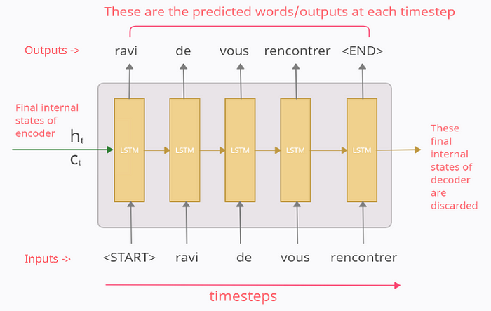
Now the way decoder works, is, that its output at any time-step t is supposed to be the tᵗʰ word in the target-sequence/Y_true (“ravi de vous rencontrer”). To explain this, let’s see what happens at each time-step.

At time-step 1

The input fed to the decoder at the first time-step is a special symbol “<START>”. This is used to signify the start of the output-sequence. Now the decoder uses this input and the internal states (hₜ, cₜ) to produce the output in the 1st time-step which is supposed to be the 1st word/token in the target-sequence i.e. ‘ravi’.

At time-step 2

At time-step 2, the output from the 1st time-step “ravi” is fed as input to the 2nd time-step. The output in the 2nd time-step is supposed to be the 2nd word in the target-sequence i.e. ‘de’

And similarly, the output at each time-step is fed as input to the next time-step. This continues till we get the “” symbol which is again a special symbol used to mark the end of the output-sequence. The final internal states of the decoder are discarded.

Note that these special symbols need not necessarily be “<START>” and “<END>” only. These can be any strings given that these are not present in our data corpus so the model doesn’t confuse them with any other word. In the paper, they have used the symbol “<EOS>” and in a slightly different manner. I will be talking a little bit more about this later.

NOTE: The process mentioned above is how an ideal decoder will work in the testing phase. But in the training phase, a slightly different implementation is required, to make it train faster. I have explained this in the next section.

3.5.1 Mathematical Foundations: Decoder

The decoder generates an output sequence:

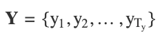
using the context vector c:

1. Initialization: The decoder’s initial hidden state s0 is set to the context vector:

2. Output Generation: For each time step t in the output sequence:

and,

where:

• st​ is the decoder’s hidden state at time t.
• fdec​ is the decoder’s activation function.
• yt−1 is the previously generated output (with y0​ being a start-of-sequence token).
• W is the weight matrix for the output layer.
• p(yt | y<t, X) is the probability distribution over the possible outputs at time t.

4. Training Encoder-Decoder Models

4.1 Vectorizing our data

Before getting into details of it, we first need to vectorize our data.

The raw data that we have is

• X = “nice to meet you” → Y_true = “ravi de vous rencontrer”

Now we put the special symbols “” and “” at the start and the end of our target-sequence

• X = “nice to meet you” → Y_true = “<START> ravi de vous rencontrer <END>”

Next the input and output data is vectorized using one-hot-encoding (ohe). Let the input and output be represented as

• X = (x1, x2, x3, x4) → Y_true = (y0_true, y1_true, y2_true, y3_true, y4_true, y5_true)

where xi’s and yi’s represent the ohe vectors for input-sequence and output-sequence respectively. They can be shown as:

For input X

‘nice’ → x1 : [1 0 0 0]

‘to’ → x2 : [0 1 0 0 ]

‘meet’ →x3 : [0 0 1 0]

‘you’ → x4 : [0 0 0 1]

For Output Y_true

‘’ → y0_true : [1 0 0 0 0 0]

‘ravi’ → y1_true : [0 1 0 0 0 0]

‘de’ → y2_true : [0 0 1 0 0 0]

‘vous’ → y3_true : [0 0 0 1 0 0]

‘rencontrer’ → y4_true : [0 0 0 0 1 0]

‘’ → y5_true : [0 0 0 0 0 1]

Note: I have used this representation for easier explanation. Both the terms ‘true sequence’ and ‘target-sequence’ have been used to refer to the same sentence “ravi de vous rencontrer” which we want our model to learn.

4.2 Training & Testing of Encoder

The working of the encoder is the same in both the training and testing phase. It accepts each token/word of the input-sequence one by one and sends the final states to the decoder. Its parameters are updated using backpropagation over time.

4.3 The Decoder in Training Phase: Teacher Forcing

The working of the decoder is different during the training and testing phase, unlike the encoder part. Hence we will see both separately.

To train our decoder model, we use a technique called “Teacher Forcing” in which we feed the true output/token (and not the predicted output/token) from the previous time-step as input to the current time-step.

To explain, let’s look at the 1st iteration of training. Here, we have fed our input-sequence to the encoder, which processes it and passes its final internal states to the decoder. Now for the decoder part, refer to the diagram below.

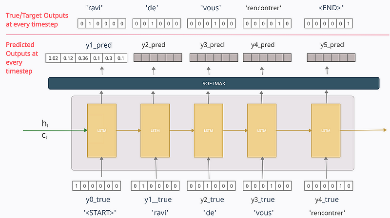
Before moving on, note that in the decoder, at any time-step t, the output yt_pred is the probability distribution over the entire vocabulary in the output dataset which is generated by using the Softmax activation function. The token with the maximum probability is chosen to be the predicted word.

For eg. referring to the above diagram, y1_pred = [0.02 0.12 0.36 0.1 0.3 0.1] tells us that our model thinks that the probability of 1st token in the output-sequence being ‘<START>’ is 0.02, ‘ravi’ is 0.12, ‘de’ is 0.36 and so on. We take the predicted word to be the one with the highest probability. Hence here the predicted word/token is ‘de’ with a probability of 0.36

Moving on…

At time-step 1

The vector [1 0 0 0 0 0] for the word ‘<START>’ is fed as the input vector. Now here I want my model to predict the output as y1_true=[0 1 0 0 0 0] but since my model has just started training, it will output something random. Let the predicted value at time-step 1 be y1_pred=[0.02 0.12 0.36 0.1 0.3 0.1] meaning it predicts the 1st token to be ‘de’. Now, should we use this y1_pred as the input at time-step 2?. We can do that, but in practice, it was seen that this leads to problems like slow convergence, model instability, and poor skill which is quite logical if we think.

Thus, teacher forcing was introduced to rectify this. in which we feed the true output/token (and not the predicted output) from the previous time-step as input to the current time-step. That means the input to the time-step 2 will be y1_true=[0 1 0 0 0 0] and not y1_pred.

Now the output at time-step 2 will be some random vector y2_pred. But at time-step 3 we will be using input as y2_true=[0 0 1 0 0 0] and not y2_pred. Similarly at each time-step, we will use the true output from the previous time-step.

Finally, the loss is calculated on the predicted outputs from each time-step and the errors are backpropagated through time to update the parameters of the model. The loss function used is the categorical cross-entropy loss function between the target-sequence/Y_true and the predicted-sequence/Y_pred such that

• Y_true = [y0_true, y1_true, y2_true, y3_true, y4_true, y5_true]
• Y_pred = [‘’, y1_pred, y2_pred, y3_pred, y4_pred, y5_pred]

The final states of the decoder are discarded.

4.4 The Decoder in Test Phase

In a real-world application, we won’t have Y_true but only X. Thus we can’t use what we did in the training phase as we don’t have the target-sequence/Y_true. Thus when we are testing our model, the predicted output (and not the true output unlike the training phase) from the previous time-step is fed as input to the current time-step. Rest is all same as the training phase.

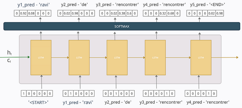
So let’s say we have trained our model and now we test it on the single sentence we trained it on. Now If we trained the model well and that too only on a single sentence then it should perform almost perfectly but for the sake of explanation say our model is not trained well or partially trained and now we test it. Let the scenario be depicted by the diagram below

At time-step 1

y1_pred = [0 0.92 0.08 0 0 0] tells that the model is predicting the 1st token/word in the output-sequence to be ‘ravi’ with a probability of 0.92 and so now at the next time-step this predicted word/token will only be used as input.

At time-step 2

The predicted word/token “ravi” from 1st time-step is used as input here. Here the model predicts the next word/token in the output-sequence to be ‘de’ with a probability of 0.98 which is then used as input at time-step 3

And the similar process is repeated at every time-step till the ‘’ token is reached

Better visualization for the same would be:

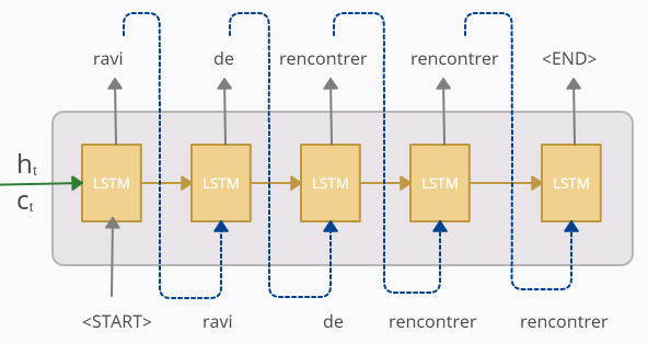
So according to our trained model, the predicted-sequence at test time is “ravi de rencontrer rencontrer”. Hence though the model was incorrect on the 3rd prediction, we still fed it as input to the next time-step. The correctness of the model depends on the amount of data available and how well it has been trained. The model may predict a wrong output but nevertheless, the same output is only fed to the next time-step in the test phase.

4.5 The Embedding Layer

One important detail I hadn’t mentioned earlier is that both the encoder and decoder process the input sequence through an embedding layer. This step reduces the dimensionality of the input word vectors, as one-hot-encoded vectors tend to be quite large in practice. Embedded vectors provide a more efficient and meaningful representation of words. For the encoder, this can be illustrated by how the embedding layer compresses the word vector dimensions, for instance, reducing them from 4 to 3.

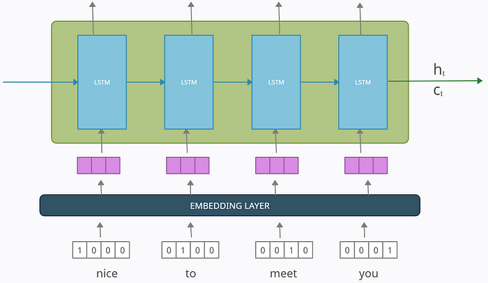
This embedding layer can be pre-trained like Word2Vec embeddings or can be trained with the model itself.

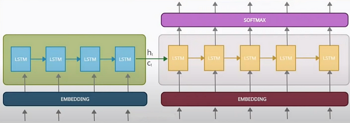
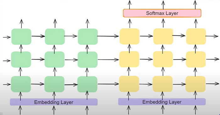
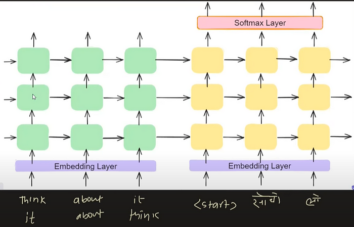
4.6 The Final Visualization at test time

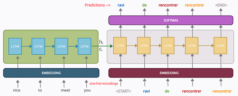
• On the left, the encoder processes the input sequence (“nice to meet you”), with each word passed through an embedding layer (to reduce dimensionality) and then through a series of LSTM layers. The encoder outputs a context vector containing hidden state ht​ and cell state ct​, summarizing the input sequence.
• On the right, the decoder receives the context vector and generates the output sequence (“ravi de rencontrer”). The decoder uses LSTMs to generate each word, taking the previous word as input (starting with a special token <START>), passing through another embedding layer, and producing predictions via a softmax layer.

The image demonstrates how the model translates an input sequence into a target sequence using embedding and recurrent layers.

5. Drawbacks of Encoder-Decoder Models

There are two primary drawbacks to this architecture, both related to length.

1. Firstly, as with humans, this architecture has minimal memory. The ultimate hidden state of the Long Short Term Memory (LSTM), S or W, is tasked with encapsulating the entire sentence for translation. Typically, S or W comprises only a few hundred units (i.e., floating-point numbers). However, cramming too much into this fixed-dimensional vector increases glossiness in the neural network. Thinking of neural net”orks in terms of the “lossy compression” they must perform is sometimes quite useful.
2. Second, as a general rule of thumb, the deeper a neural network is, the harder it is to train. For recurrent neural networks, the longer the sequence is, the deeper the neural network is along the time dimension. This results in vanishing gradients, where the gradient signal from the objective that the recurrent neural network learns from disappears as it travels backward. Even with RNNs specifically made to help prevent vanishing gradients, such as the LSTM, this is still a fundamental problem.

Furthermore, we have models like Attention Models and Transformers for more robust and lengthy sentences.

6. Improvements in Encoder-Decoder Architecture

6.1 Adding Embedding Layer

The embedding layer converts input tokens into dense vector representations, allowing the model to learn meaningful representations of words or tokens in the input sequence.

By using a trainable embedding layer and exploring techniques such as pre-trained word embeddings or contextual embeddings, we can enrich the input representations, enabling the model to capture nuanced semantic and syntactic information more effectively. This enhancement facilitates better understanding and generation of sequential data.

6.2 Use of Deep LSTMs

LSTMs are recurrent neural network (RNN) variants known for their ability to capture long-range dependencies in sequential data. Deepening the LSTM layers enables the model to learn hierarchical representations of the input and output sequences, leading to improved performance.

Increasing the depth of the LSTM layers and incorporating techniques like residual connections or layer normalization help mitigate issues like vanishing gradients and facilitate the training of deeper networks. These enhancements empower the model to learn more complex patterns and dependencies in the data, resulting in better sequence generation and understanding.

6.3 Reverse the input

Reversing the input sequence in machine translation, such as English to Hindi or English to French conversion, has been shown to enhance model performance in some cases by aiding in capturing long-range dependencies and mitigating vanishing gradient issues.

However, its effectiveness can vary depending on linguistic characteristics and dataset complexity, and it may not consistently improve performance across all scenarios. Careful evaluation and experimentation are necessary to determine whether reversing the input sequence is beneficial for a specific task and dataset.

We now understand the concept of Encoder Decoder. Now, If we go through the famous research paper “Sequence to Sequence Learning with Neural Networks,” by Ilya Sutskever, then we will understand the paper concept very well. Below I summarize what is inside the paper :

1. Application to Translation: The model focused on translating English to French, demonstrating the effectiveness of sequence-to-sequence learning in neural machine translation.
2. Special End-of-Sentence Symbol: Each sentence in the dataset was terminated with a unique end-of-sentence symbol (“”), enabling the model to recognize the end of a sequence.
3. Dataset: The model was trained on a subset of 12 million sentences, comprising 348 million French words and 304 million English words, taken from a publicly available dataset.
4. Vocabulary Limitation: To manage computational complexity, fixed vocabularies for both languages were used, with 160,000 most frequent words for English and 80,000 for French. Words not in these vocabularies were replaced with a special “UNK” token.
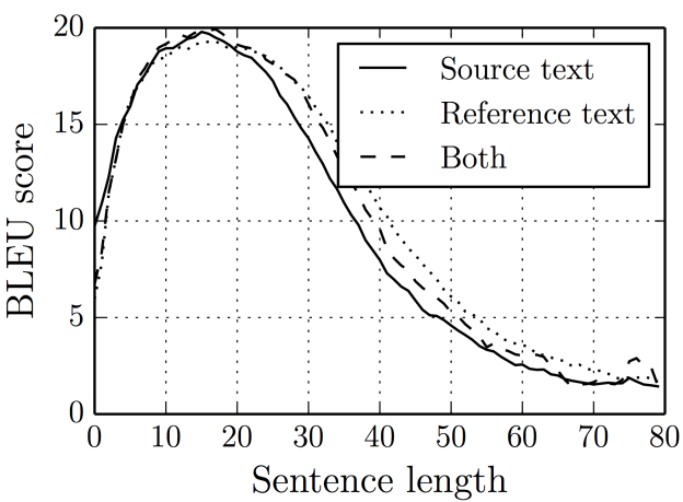
5. Reversing input sequences: The input sentences were reversed before feeding them into the model, which was found to significantly improve the model’s learning efficiency, especially for longer sentences.
6. Word Embeddings: The model used a 1000-dimensional word embedding layer to represent input words, providing dense, meaningful representations of each word.
7. Architecture Details: Both the input(encoder) and output(decoder) models had 4 layers, with each layer containing 1000 units, showcasing a deep LSTM-based architecture.
8. Output Layer and Training: The output layer employed a SoftMax function to generate the probability distribution over the largest vocabulary. The model was trained end to end with these settings.
9. Performance — BLEU Score: The model achieved a BLEU score of 34.81, surpassing the base file Statistical Machine Translation system’s score of 33.30 on the same dataset, marking a significant advancement in neural machine translation.

7. Example: Encoder-Decoder Architecture with Neural Networks

We can use CNN, RNN & LSTM in encoder-decoder architecture to solve different kinds of problems. Using a combination of different types of networks can help to capture the complex relationships between the input and output sequence of data. Here are different scenarios or problem examples where CNN, RNN, LSTM, transformer, etc. can be used:

• CNN as Encoder, RNN/LSTM as Decoder: This architecture can be used for tasks like image captioning, where the input is an image and the output is a sequence of words describing the image. The CNN can extract features from the image, while the RNN/LSTM can generate the corresponding text sequence. Recall that CNNs are good at extracting features from images and this is why they can be used as the encoder in tasks that involve images. Also, RNNs/LSTMs are good at processing sequential data such as sequences of words, and can be used as the decoder in tasks that involve text sequences.
• RNN/LSTM as Encoder, RNN/LSTM as Decoder: This architecture can be used for tasks like machine translation, where the input and output are both sequences of words of varying length. The RNN/LSTM in the encoder can encode the input sequence of words into a hidden state or numerical representation, while the RNN/LSTM in the decoder can generate the corresponding output sequence of words in different languages. The picture below represents encoder-decoder architecture with RNN used in both encoder and decoder networks. The sequence of words as input is in English and the output is machine translation in German.

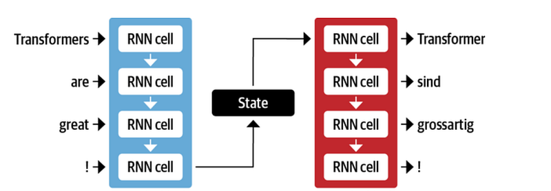
• There is a disadvantage to using RNNs in encoder-decoder architecture. The final numerical representation or hidden state in the encoder network has to represent the entire context and meaning of a sequence of data. If the sequence of data is long enough, it may get challenging and the information about the start of the sequence might get lost in the process of compressing entire information in the form of numerical representation.

There are a few limitations one needs to keep in mind when using different types of neural networks such as CNN, RNN, LSTM, etc in encoder-decoder architecture:

• CNNs can be computationally expensive and may require a lot of training data.
• RNNs/LSTMs can suffer from vanishing/exploding gradients and may require careful initialization and regularization.
• Using a combination of different types of networks can make the model more complex and difficult to train.

8. Applications of Encoder-Decoder Neural Network Architecture

The following are some of the real-life/real-world applications of encoder-decoder neural network architecture:

• Transformer models: The Transformer model, as originally proposed in the paper “Attention Is All You Need” by Vaswani et al., consists of both an encoder and a decoder. Each part is composed of layers that use self-attention mechanisms. The encoder processes the input data (like text) and creates context-rich representations of it. The decoder uses these representations along with its inputs (like the previous word in a sentence) to generate an output sequence. T5 (Text-To-Text Transfer Transformer) utilizes an encoder-decoder architecture. Then, there is another example of BART (Bidirectional and Auto-Regressive Transformers) that combines a bidirectional encoder (like BERT) with an autoregressive decoder (like GPT).
• Make-a-Video: Recently introduced AI system by Facebook / Meta namely Make-a-Video is likely powered by deep learning techniques, possibly including an encoder-decoder architecture for translating text prompts into video content. This architecture, commonly used in sequence-to-sequence transformations, would use an encoder to convert input text into a dense vector representation, and a decoder to transform this vector into video content. However, given the complexity of creating video from text, the system might also employ advanced generative models like Generative Adversarial Networks (GANs) or Variational Autoencoders (VAEs), which excel in generating high-quality, realistic images. Further, to learn mappings from text to visuals and understand the dynamics of the world, it likely leverages large amounts of paired text-image data and video footage, possibly employing unsupervised learning or self-supervised learning techniques.
• Machine translation: One of the most common applications of the Encoder-Decoder architecture is Machine Translation. This is where a sequence of words in one language as shown above (encoder-decoder architecture with RNN) is translated into another language. The Encoder-Decoder model can be trained on a large corpus of bilingual texts to learn how to map a sequence of words in one language to the equivalent sequence in another language.
• Image captioning: Image captioning is another application of encoder-decoder architecture. This is where an image is processed by an encoder (using CNN), and the output is passed to a decoder (RNN or LSTM) that generates a textual description of the image. This can be used for applications like automatic image tagging and captioning.

9. Sequence-to-Sequence Learning with Neural Networks (Hands-On)

In this tutorial, we’ll walk through how to implement a basic sequence-to-sequence (Seq2Seq) model using an Encoder-Decoder architecture in PyTorch. The Seq2Seq model is widely used for tasks like machine translation, text summarization, and question answering. It works by taking in a sequence (like a sentence) as input and generating a sequence (like a translated sentence) as output.

We’ll use a simplified machine translation task, translating German to English, using the `Multi30k` dataset.

What is the Multi30k Dataset?

The `Multi30k` dataset is a collection of parallel English-German sentences. Each sentence in the dataset is a pair of a sentence in German and its corresponding translation in English. This dataset is often used for training machine translation models.

For our model, we will tokenize the sentences, build vocabularies for both languages, and train the model to translate German sentences into English.

Project Overview

1. Data Preprocessing: We’ll tokenize sentences in German and English and prepare the dataset for training. 2. Model Architecture: We’ll create two components: — Encoder: Reads the source (German) sentence and converts it into a context vector. — Decoder: Uses the context vector to generate the target (English) sentence. 3. Training: Train the model on the dataset to minimize the loss between the predicted and actual target sentences. 4. Evaluation: We’ll evaluate the model by translating new sentences and computing the BLEU score, which is commonly used to evaluate the quality of machine translations.

Step 1: Installing and Importing Libraries

We’ll use a few libraries: `torch` for deep learning, `torchtext` for handling datasets, and `spacy` for tokenization.

Install the required libraries using:

pip install torch torchtext spacy
python -m spacy download de_core_news_sm
python -m spacy download en_core_web_sm

Next, import the libraries:

import torch
import torch.nn as nn
import torch.optim as optim
import random
import spacy
from torchtext.data import Field, BucketIterator
from torchtext.datasets import Multi30k

Step 2: Data Preprocessing

We’ll use the `Multi30k` dataset, which provides sentence pairs in English and German. The German sentences will be reversed to help the model learn better alignment between source and target sentences.

Tokenization

To split the sentences into words, we’ll use `spacy`:

spacy_de = spacy.load('de_core_news_sm')
spacy_en = spacy.load('en_core_web_sm')
def tokenize_de(text):
 return [tok.text for tok in spacy_de.tokenizer(text)][::-1]
def tokenize_en(text):
 return [tok.text for tok in spacy_en.tokenizer(text)]

Field Definitions

We use `torchtext`’s `Field` to define how the data will be processed. We specify how to tokenize the data and handle the start (``) and end (``) tokens.

SRC = Field(tokenize=tokenize_de, init_token='<sos>', eos_token='<eos>', lower=True)
TRG = Field(tokenize=tokenize_en, init_token='<sos>', eos_token='<eos>', lower=True)

Loading and Building Vocab

We now load the dataset and build the vocabulary for the source (German) and target (English) languages.

train_data, valid_data, test_data = Multi30k.splits(exts=('.de', '.en'), fields=(SRC, TRG))
SRC.build_vocab(train_data, min_freq=2)
TRG.build_vocab(train_data, min_freq=2)

`min_freq=2` ensures that only words that appear at least twice in the training data are included in the vocabulary.

Step 3: Building the Encoder

The Encoder is an RNN that reads a sequence of words (in this case, a German sentence) and encodes it into a context vector.

class Encoder(nn.Module):
 def __init__(self, input_dim, emb_dim, hid_dim, n_layers, dropout):
 super().__init__()
 self.embedding = nn.Embedding(input_dim, emb_dim)
 self.rnn = nn.GRU(emb_dim, hid_dim, n_layers, dropout=dropout)
 self.dropout = nn.Dropout(dropout)
 
 def forward(self, src):
 # src = [src_len, batch_size]
 embedded = self.dropout(self.embedding(src)) # [src_len, batch_size, emb_dim]
 outputs, hidden = self.rnn(embedded)
 return hidden

- input_dim: The size of the source vocabulary. - emb_dim: Embedding dimension (converts each word into a fixed-size vector). - hid_dim: Hidden dimension of the GRU (number of units in each layer of the RNN). - n_layers: Number of GRU layers. - dropout: Regularization to prevent overfitting.

Step 4: Building the Decoder

The Decoder generates the target sentence (in English) one word at a time, conditioned on the context vector produced by the encoder.

class Decoder(nn.Module):
 def __init__(self, output_dim, emb_dim, hid_dim, n_layers, dropout):
 super().__init__()
 self.embedding = nn.Embedding(output_dim, emb_dim)
 self.rnn = nn.GRU(emb_dim, hid_dim, n_layers, dropout=dropout)
 self.fc_out = nn.Linear(hid_dim, output_dim)
 self.dropout = nn.Dropout(dropout)
 
 def forward(self, input, hidden):
 # input = [batch_size]
 input = input.unsqueeze(0) # [1, batch_size]
 embedded = self.dropout(self.embedding(input)) # [1, batch_size, emb_dim]
 output, hidden = self.rnn(embedded, hidden) # [1, batch_size, hid_dim], [n_layers, batch_size, hid_dim]
 prediction = self.fc_out(output.squeeze(0)) # [batch_size, output_dim]
 return prediction, hidden

- output_dim: Size of the target vocabulary (English). - embedding: Converts words into vectors. - fc_out: Fully connected layer to map hidden states to the output vocabulary.

Step 5: Building the Seq2Seq Model

The Seq2Seq model brings together the Encoder and Decoder. It uses the Encoder to encode the source sequence into a context vector, and the Decoder to generate the target sequence.

class Seq2Seq(nn.Module):
 def __init__(self, encoder, decoder, device):
 super().__init__()
 self.encoder = encoder
 self.decoder = decoder
 self.device = device
def forward(self, src, trg, teacher_forcing_ratio=0.5):
 trg_len = trg.shape[0]
 batch_size = trg.shape[1]
 trg_vocab_size = self.decoder.fc_out.out_features
 
 outputs = torch.zeros(trg_len, batch_size, trg_vocab_size).to(self.device)
 hidden = self.encoder(src)
 
 input = trg[0, :]
 for t in range(1, trg_len):
 output, hidden = self.decoder(input, hidden)
 outputs[t] = output
 top1 = output.argmax(1)
 input = trg[t] if random.random() < teacher_forcing_ratio else top1
 
 return outputs

- teacher_forcing_ratio: Determines whether to use the actual target token or the predicted token as the next input during training (helpful to stabilize training). - outputs: Stores the predictions at each time step.

Step 6: Training the Model

We define the training loop, where we feed in the German sentence, run it through the Seq2Seq model, and compute the loss using Cross Entropy.

def train(model, iterator, optimizer, criterion, clip):
 model.train()
 epoch_loss = 0
 
 for i, batch in enumerate(iterator):
 src = batch.src
 trg = batch.trg
 
 optimizer.zero_grad()
 output = model(src, trg)
 
 output_dim = output.shape[-1]
 output = output[1:].view(-1, output_dim)
 trg = trg[1:].view(-1)
 
 loss = criterion(output, trg)
 loss.backward()
 torch.nn.utils.clip_grad_norm_(model.parameters(), clip)
 optimizer.step()
 epoch_loss += loss.item()
 
 return epoch_loss / len(iterator)

- Gradient Clipping: Used to prevent exploding gradients. - Cross Entropy Loss: Measures the error between the predicted and actual tokens.

Step 7: Evaluate the Model

Evaluation works similarly to training, but we disable backpropagation since we’re only interested in the model’s performance.

def evaluate(model, iterator, criterion):
 model.eval()
 epoch_loss = 0
 
 with torch.no_grad():
 for i, batch in enumerate(iterator):
 src = batch.src
 trg = batch.trg
 output = model(src, trg, 0)
 
 output_dim = output.shape[-1]
 output = output[1:].view(-1, output_dim)
 trg = trg[1:].view(-1)
loss = criterion(output, trg)
 epoch_loss += loss.item()
 
 return epoch_loss / len(iterator)

Step 8: Initialize the Model and Hyperparameters

Now, we initialize the model, optimizer, and loss function, and specify hyperparameters.

INPUT_DIM = len(SRC.vocab)
OUTPUT_DIM = len(TRG.vocab)
ENC_EMB_DIM = 256
DEC_EMB_DIM = 256
HID_DIM = 512
N_LAYERS = 2
ENC_DROPOUT = 0.5
DEC_DROPOUT = 0.5

enc = Encoder(INPUT_DIM, ENC_EMB_DIM, HID_DIM, N_LAYERS, ENC_DROPOUT)
dec = Decoder(OUTPUT_DIM, DEC_EMB_DIM, HID_DIM, N_LAYERS, DEC_DROPOUT)

device = torch.device('cuda' if torch.cuda.is_available() else 'cpu')
model = Seq2Seq(enc, dec, device).to(device)
optimizer = optim.Adam(model.parameters())
TRG_PAD_IDX = TRG.vocab.stoi[TRG.pad_token]
criterion = nn.CrossEntropyLoss(ignore_index=TRG_PAD_IDX)

Step 9: Training Loop

We train the model for a set number of epochs.

N_EPOCHS = 10
CLIP = 1

for epoch in range(N_EPOCHS):
 train_loss = train(model, train_iterator, optimizer, criterion, CLIP)
 valid_loss = evaluate(model, valid_iterator, criterion)
 
 print(f'Epoch: {epoch+1}')
 print(f'Train Loss: {train_loss:.3f} | Val. Loss: {valid_loss:.3f}')

Step 10: Testing with BLEU Score

Finally, we can test our model by translating new sentences and evaluating the BLEU score.

def translate_sentence(sentence, src_field, trg_field, model, device, max_len=50):
 model.eval()
 tokens = [token.text.lower() for token in spacy_de(sentence)]
 tokens = [src_field.init_token] + tokens + [src_field.eos_token]
 
 src_indexes = [src_field.vocab.stoi[token] for token in tokens]
 src_tensor = torch.LongTensor(src_indexes).unsqueeze(1).to(device)
 
 with torch.no_grad():
 hidden = model.encoder(src_tensor)
 
 trg_indexes = [trg_field.vocab.stoi[trg_field.init_token]]
 for i in range(max_len):
 trg_tensor = torch.LongTensor([trg_indexes[-1]]).to(device)
 with torch.no_grad():
 output, hidden = model.decoder(trg_tensor, hidden)
 pred_token = output.argmax(1).item()
 trg_indexes.append(pred_token)
 if pred_token == trg_field.vocab.stoi[trg_field.eos_token]:
 break
 trg_tokens = [trg_field.vocab.itos[i] for i in trg_indexes]
 return trg_tokens[1:]

This function translates a sentence from German to English using the trained Seq2Seq model.

10. Conclusion

In this blog, we explored sequence modeling through the powerful Encoder-Decoder architecture. Starting with the challenges of sequential data, we discussed how this architecture efficiently handles sequence-to-sequence tasks, such as neural machine translation. We delved into the encoder’s role in capturing input information and the decoder’s function in generating coherent output, backed by their mathematical foundations.

We also covered training techniques like teacher forcing, practical implementation steps, and explored the “Sutskever Model” as a real-world application of the Encoder-Decoder approach. The hands-on example provided a step-by-step guide to building and evaluating a sequence-to-sequence model.

With applications extending beyond translation, this architecture is widely used in text summarization, speech recognition, and more. By mastering both its theory and practical use, we can leverage the Encoder-Decoder architecture to solve a variety of complex problems across different domains.

11. Test your Knowledge!

1. How does the use of bidirectional LSTMs in the encoder improve the performance of a Seq2Seq model?

— Expected Answer: Bidirectional LSTMs process the input sequence in both forward and backward directions, capturing more context from both past and future states. This helps the encoder build a more comprehensive representation of the input sequence, leading to better performance in downstream tasks like translation or summarization.

2. Describe how you would implement a Seq2Seq model for a real-time translation system. What challenges might you face?

— Expected Answer: A real-time translation system requires low latency, making it essential to optimize the model for speed without compromising accuracy. Challenges include handling varying sentence lengths, maintaining context, and ensuring fluency in the target language. Techniques like attention mechanisms and beam search can help, but they must be carefully tuned to balance accuracy and speed.

3. Explain how attention mechanisms differ from traditional Seq2Seq models and how they handle long sequences.

— Expected Answer: Traditional Seq2Seq models compress the input sequence into a fixed-size vector, which can lead to information loss, especially with long sequences. Attention mechanisms address this by allowing the model to focus on specific parts of the input sequence when generating each word of the output, dynamically adjusting the “focus” based on the context, thus handling long sequences more effectively.

4. In what scenarios would you prefer Transformer models over traditional RNN-based Seq2Seq models?

— Expected Answer: Transformers are preferred when dealing with very long sequences or when parallelization is critical, as they do not rely on sequential processing like RNNs. They are also effective in capturing long-range dependencies through self-attention mechanisms, making them suitable for tasks like language modeling, translation, and even non-language tasks like image processing.

5. What is the role of positional encoding in Transformer models, and why is it necessary?

— Expected Answer: Positional encoding in Transformer models provides the model with information about the position of each token in the sequence since Transformers process the input in parallel rather than sequentially. This encoding allows the model to capture the order of tokens, which is crucial for understanding the structure and meaning of the input sequence.

6. How would you handle the problem of overfitting in a Seq2Seq model?

— Expected Answer: Overfitting in Seq2Seq models can be mitigated by techniques such as regularization (e.g., L2 regularization, dropout), using a larger dataset, data augmentation, early stopping, and employing more sophisticated architectures like attention mechanisms that improve generalization. Additionally, monitoring validation loss and adjusting model complexity as needed can help prevent overfitting.

7. Can you discuss the trade-offs between using beam search and greedy search in Seq2Seq models?

— Expected Answer: Greedy search selects the most probable word at each step, which is faster but may miss the globally optimal sequence. Beam search, on the other hand, considers multiple potential sequences at each step (beam width) and is more likely to find the optimal sequence but at the cost of increased computational complexity. The choice depends on the application’s needs for accuracy versus speed.

8. How would you modify a Seq2Seq model to handle a multi-lingual translation task?

— Expected Answer: For a multi-lingual translation task, you can introduce a shared encoder and multiple decoders, each corresponding to a different target language, or use a single decoder with a special token indicating the target language. Fine-tuning the model on multiple languages and incorporating transfer learning can also improve performance across languages.

9. Describe how you would implement a Seq2Seq model for a chatbot application. What are the key considerations?

— Expected Answer: Implementing a Seq2Seq model for a chatbot involves ensuring the model can generate coherent and contextually appropriate responses. Key considerations include handling multi-turn conversations, maintaining context across interactions, ensuring diversity in responses, and minimizing biases in generated text. Incorporating reinforcement learning or fine-tuning with human feedback can enhance the chatbot’s effectiveness.

10. What are the limitations of Seq2Seq models in handling tasks like text summarization or translation, and how can they be addressed?

— Expected Answer: Seq2Seq models may struggle with maintaining coherence, handling long sequences, and producing grammatically correct output. These limitations can be addressed by using attention mechanisms, incorporating larger and more diverse datasets, employing pre-trained models like BERT or GPT, and fine-tuning on specific tasks. Evaluation metrics like BLEU and ROUGE can help assess and improve performance.

11. Do the encoder and the decoder have to be the same type of neural network?

— Expected Answer: No, the encoder and decoder do not have to be the same type of neural network. In many implementations, both are RNNs (e.g., LSTMs or GRUs), but they can differ based on the task’s requirements. For example, the encoder could be a Convolutional Neural Network (CNN) for processing images, while the decoder could be an RNN for generating sequences. The key requirement is that the output of the encoder should be compatible with the input of the decoder.

12. Besides machine translation, can you think of another application where the encoder–decoder architecture can be applied?

— Expected Answer: Yes, the encoder-decoder architecture can be applied to various tasks, including text summarization. In text summarization, the encoder processes the input document and creates a condensed representation, while the decoder generates a shorter version that captures the key information. Other applications include image captioning (where the encoder is a CNN processing the image and the decoder is an RNN generating the caption) and speech recognition (where the encoder processes audio signals and the decoder generates the corresponding text).

13. What is “Teacher Forcing” in the context of training a decoder in an Encoder-Decoder model, and why is it used? Discuss any potential drawbacks of this approach.

— Expected Answer: Teacher Forcing is a training technique where the actual target output is used as the next input to the decoder instead of the model’s prediction. It speeds up convergence and improves learning by providing the correct context at each step.

14. How does an encoder process an input sequence mathematically?

— Expected Answer: At each time step t, the encoder updates its hidden state using ht=f(et,ht−1), where et is the embedded input and f is a recurrent function like an LSTM or GRU.

15. Discuss the role of the embedding layer during the test phase of the decoder. How does it differ from its role during training, if at all?

— Expected Answer: The embedding layer converts tokens into dense vector representations that capture semantic relationships, allowing the model to process and learn from textual data more effectively.

16. Provide an example of how an Encoder-Decoder architecture can be applied outside of machine translation. Describe the problem and how the architecture addresses it.

— Expected Answer: In text summarization, the Encoder-Decoder model condenses a lengthy document (encoder) into a brief summary (decoder), effectively capturing the main points.

17. What are the mathematical foundations of the decoder block in an Encoder-Decoder architecture? Explain how the decoder generates the output sequence.

— Expected Answer: The decoder computes st=f(et,st−1,c) at each step, where et​ is the embedding of the previous token, st−1​ is the previous state, and ccc is the context vector, then predicts the next token.

18. Suppose that we use neural networks to implement the encoder-decoder architecture. Do the encoder and the decoder have to be the same type of neural network?

— Expected Answer: No, the encoder and decoder do not have to be the same type of neural network. For example, in practical applications like image captioning, a Convolutional Neural Network (CNN) is often used as the encoder to process the image, while a Recurrent Neural Network (RNN) or Transformer is used as the decoder to generate the descriptive text.

Thank you for reading!

If this guide has enhanced your understanding of Python and Machine Learning:

• Please show your support with a clap 👏 or several claps!
• Your claps help me create more valuable content for our vibrant Python or ML community.
• Feel free to share this guide with fellow Python or AI / ML enthusiasts.
• Your feedback is invaluable — it inspires and guides my future posts.

Connect with me!

Vipra