LLM Architectures Explained: RNNs, LSTMs & GRUs (Part 3)

Deep Dive into the architecture & building real-world applications leveraging NLP Models starting from RNN to Transformer.

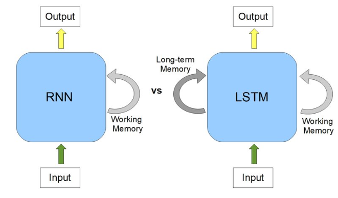
Posts in this Series

1. NLP Fundamentals
2. Word Embeddings
3. RNNs, LSTMs & GRUs ( This Post )
4. Encoder-Decoder Architecture
5. Attention Mechanism
6. Transformers
7. BERT
8. GPT
9. LLama
10. Mistral

Table of Contents

· 1. What is a Neural Network? ∘ 1.1 How do neural networks learn? ∘ 1.2 Epochs, Batch Size & Iterations ∘ 1.3 Types of Neural Networks · 2. Recurrent Neural Networks (RNNs) ∘ 2.1 What is Sequential data? ∘ 2.2 Recurrent Neural Networks vs. Feedforward Neural Networks ∘ 2.3 Why use RNNs ? · 3. The Architecture of RNNs ∘ 3.1 Unfolding RNNs in Time ∘ 3.2 Key Operations in RNNs ∘ 3.2.1 Forward Pass ∘ 3.2.2 Backpropagation Through Time (BPTT) ∘ 3.2.3 Weight Updates · 4. Challenges in Training RNNs ∘ 4.1 What is Vanishing Gradient? ∘ 4.2 What is Exploding Gradient? ∘ 4.3 Why Do the Gradients Even Vanish/Explode? ∘ 4.4 How to Know if Our Model is Suffering From the Exploding/Vanishing Gradient Problem? · 5. Handle Vanishing/Exploding Gradients ∘ 5.1 Proper Weight Initialization ∘ Wait, but how do we put these strategies into code ?? ∘ 5.2 Using Non-saturating Activation Functions ∘ 5.3 Batch Normalization ∘ 5.4 Gradient Clipping · 6. Building RNN from Scratch ∘ 6. 1 Defining the RNN Class ∘ 6.2 Early Stopping Mechanism ∘ 6.3 RNN Trainer Class ∘ 6.4 Data Loading and Preprocessing ∘ 6.5 Training the RNN · 7. Long Short-Term Memory Networks (LSTMs) · 8. LSTM Architecture ∘ 8.1 Activation Functions and Linear Operations ∘ 8.2 The Key Concepts Behind the LSTM Algorithm ∘ 8.2.1 Forget Gate ∘ 8.2.2 Input Gate ∘ 8.2.3 Output Gate · 9. Working Procedure of LSTM · 10. Types of LSTM Architectures · 11. Building an LSTM from Scratch in Python ∘ 11.1 Imports and Initial Setup ∘ 11.2 LSTM Class ∘ 11.3 Training and Validation ∘ 11.4 Data Preprocessing ∘ 11.5 Model Training · 12. Gated Recurrent Units (GRUs) ∘ 12.1 Comparison with LSTMs and Vanilla RNNs ∘ 12.2 What makes GRU special and more effective than traditional RNN? ∘ 12.2.1 Update Gate ∘ 12.2.2 Reset Gate · 13. Gates in Action · 14. Implementation of a Simple GRU · 14.1 Pros and Cons of GRUs ∘ 14.2 Choosing Between GRUs and LSTMs · 15. Conclusion · 16. Test your Knowledge!

1. What is a Neural Network?

A neural network, or artificial neural network, is a computing architecture based on a model of how a human brain functions — hence the name “neural.” Neural networks comprise a collection of processing units called “nodes.” These nodes pass data to each other, just like how in a brain, neurons pass electrical impulses to each other.

Neural networks are used in machine learning, which refers to a category of computer programs that learn without definite instructions. Specifically, neural networks are used in deep learning — an advanced type of machine learning that can draw conclusions from unlabeled data without human intervention. For instance, a deep learning model built on a neural network and fed sufficient training data could be able to identify items in a photo it has never seen before.

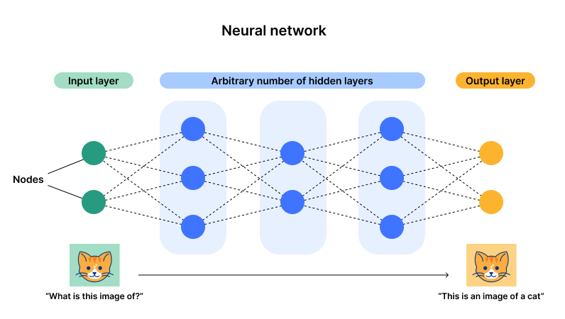
Neural networks make many types of artificial intelligence (AI) possible. Large language models (LLMs) such as ChatGPT, AI image generators like DALL-E, and predictive AI models all rely to some extent on neural networks.

1.1 How do neural networks learn?

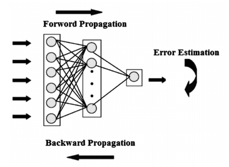
The learning (training) process of a neural network is an iterative process in which the calculations are carried out forward and backward through each layer in the network until the loss function is minimized.

The entire learning process can be divided into three main parts:

• Forward propagation (Forward pass)
• Calculation of the loss function
• Backward propagation (Backward pass/Backpropagation)

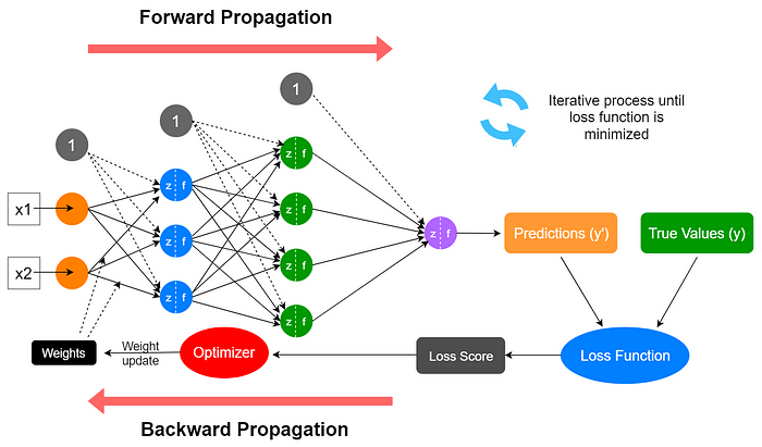
We’ll begin with forward propagation.

Forward propagation

A neural network is made of multiple neurons (perceptrons) and these neurons are stacked into layers. The connections between the layers occurred through the parameters (represented by arrows) of the network. The parameters are weights and biases.

The weights control the level of importance of each input while biases determine how easily a neuron fires or activates.

First, we assign non-zero random values to weights and biases. This is called parameter initialization of the network. Based on these assigned values and the input values, we perform the following calculations in each neuron of the network.

• Calculation of neuron’s linear function
• Calculation of neuron’s activation function

These calculations occur throughout the entire network. After completing the calculations in the output layer node(s), we get the final output of the forward propagation part in the first iteration.

In forward propagation, calculations are made from the input layer to the output layer (left to right) throughout the network.

Calculation of the loss function

The final output performed in the forward propagation is called the predicted value. This value should be compared with the corresponding ground-truth value (real value) to measure the performance of the neural network. This is where the loss function (also called objective function or cost function) comes into play.

In the context of neural networks, the cost function and the loss function are related but refer to different aspects of the model’s performance evaluation.

The loss function measures the error on a single example, and the cost function aggregates this error across the whole dataset to guide training.

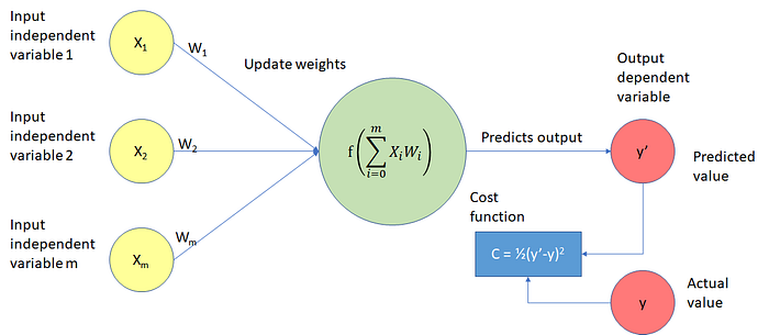
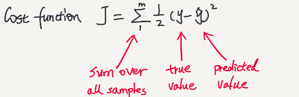
The loss function computes a score called the loss score between the predicted values and ground truth values. This is also known as the error of the model. The loss function captures how well the model performs in each iteration. We use the loss score as a feedback signal to update parameters in the backpropagation part.

The ideal value of the loss function is zero (0). Our goal is to minimize the loss function close to 0 in each iteration so that the model will make better predictions that are close to ground truth values.

Here is a list of commonly used loss functions in neural network training.

• Mean Squared Error (MSE) — This is used to measure the performance of regression problems.
• Mean Absolute Error (MAE) — This is used to measure the performance of regression problems.
• Mean Absolute Percentage Error — This is used to measure the performance of regression problems.
• Huber Loss — This is used to measure the performance of regression problems.
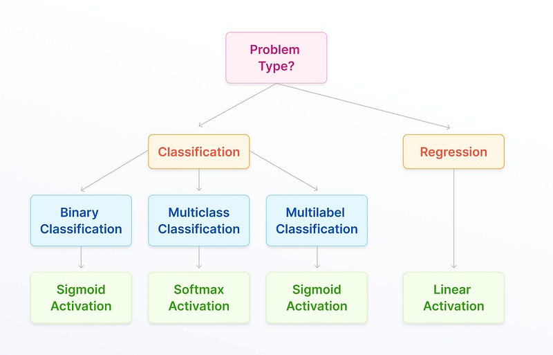
• Binary Cross-entropy (Log Loss) — This is used to measure the performance of binary (two-class) classification problems.
• Multi-class Cross-entropy/Categorical Cross-entropy — This is used to measure the performance of multi-class (more than two classes) classification problems.

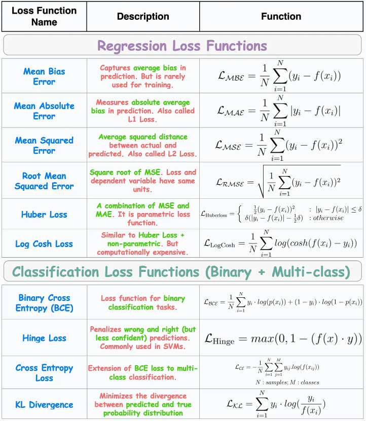
A complete list of available loss functions in Keras can be found here.

Backward propagation

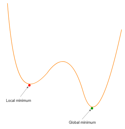
In the first iteration, the predicted values are far from the ground truth values and the distance score will be high. This is because we initially assigned arbitrary values to the network’s parameters (weights and biases). Those values are not optimal values. So, we need to update the values of these parameters in order to minimize the loss function. The process of updating network parameters is called parameter learning or optimization which is done using an optimization algorithm (optimizer) that implements backpropagation.

The objective of the optimization algorithm is to find the global minima where the loss function has its minimum value. However, it is a real challenge for an optimization algorithm to find the global minimum of a complex loss function by avoiding all the local minima. If the algorithm is stopped at a local minimum, we’ll not get the minimum value for the loss function. Therefore, our model will not perform well.

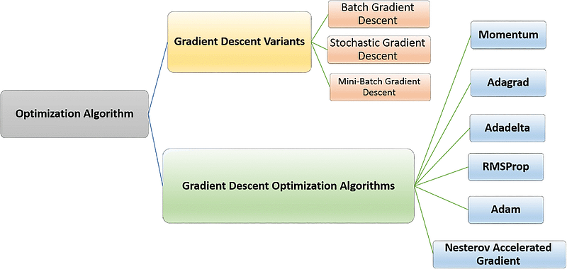
Here is a list of commonly used optimizers in neural network training.

• Gradient Descent
• Stocasticc Gradeint Descent (SGD)
• Adam
• Adagrad
• Adadelta
• Adamax
• Nadam
• Ftrl
• Root Mean Squared Propagation (RMSProp)

In the backward propagation, the partial derivatives (gradients) of the loss function with respect to the model parameters in each layer are calculated. This is done by applying the chain rule of calculus.

The derivative of the loss function is its slope which provides us with the direction that we should need to consider for updating (changing) the values of the model parameters.

The neural network libraries in Keras provide automatic differentiation. This means, after you define the neural network architecture, the libraries automatically calculate all of the derivates needed for backpropagation.

In the backward propagation, calculations are made from the output layer to the input layer (right to left) through the network.

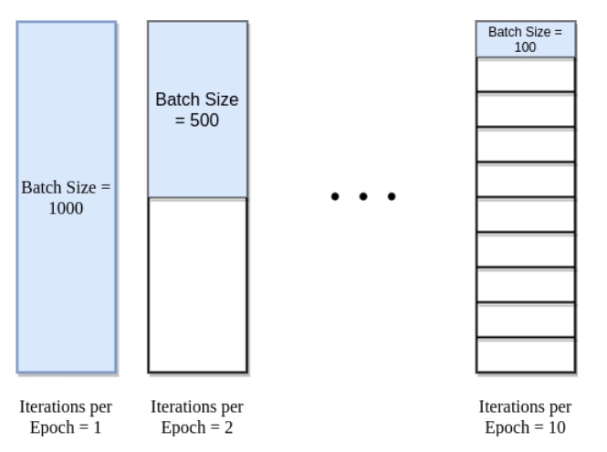
1.2 Epochs, Batch Size & Iterations

Epochs

One Epoch is when an ENTIRE dataset is passed forward and backward through the neural network only ONCE.

Since one epoch is too big to feed to the computer at once we divide it into several smaller batches.

Batch Size

The total number of training examples present in a single batch.

Note: Batch size and number of batches are two different things.

But What is a Batch?

We cannot pass the entire dataset into the neural net at once. So, we divide the dataset into a number of Batches or sets or parts.

Iterations

Iterations are the number of batches needed to complete one epoch.

Note: The number of batches is equal to the number of iterations for one epoch.

Let’s say we have 1000 training examples that we are going to use . We can divide the dataset of 1000 examples into batches of 500 then it will take 2 iterations to complete 1 epoch where Batch Size is 500 and Iterations is 2, for 1 complete epoch (case 2 in the below image).

We do not usually use all training samples (instances/rows) in one iteration during the neural network training. Instead, we specify the batch size which determines the number of training samples to be propagated (forward and backward) during training.

1.3 Types of Neural Networks

There is no limit on how many nodes and layers a neural network can have, and these nodes can interact in almost any way. Because of this, the list of types of neural networks is ever-expanding. But, they can roughly be sorted into these categories:

• Shallow neural networks (usually have only one hidden layer)
• Deep neural networks (have multiple hidden layers)

Shallow neural networks are fast and require less processing power than deep neural networks, but they cannot perform as many complex tasks as deep neural networks.

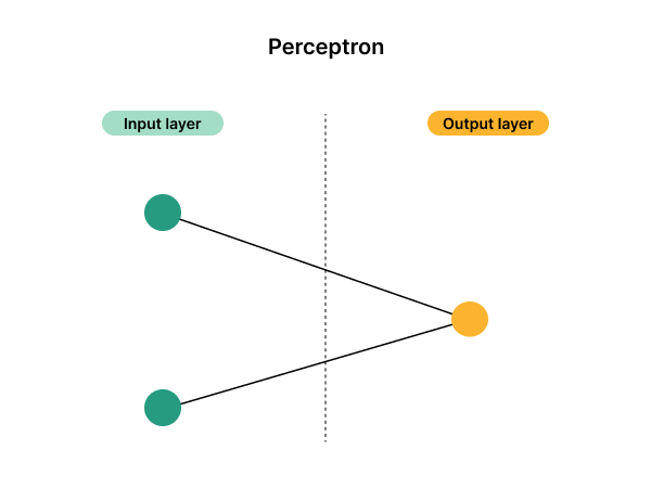
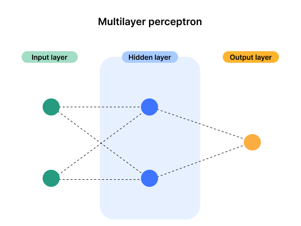
Below is a list of the types of neural network architectures that may be used today:

Perceptron neural networks are simple, shallow networks with an input layer and an output layer.

Multilayer perceptron neural networks add complexity to perceptron networks, and include a hidden layer.

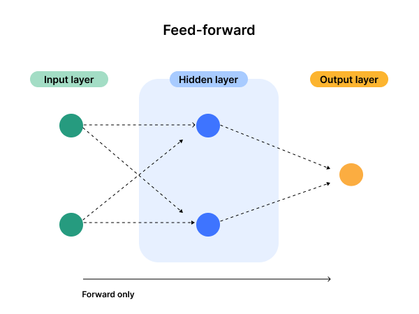
Feed-forward neural networks only allow their nodes to pass information to a forward node.

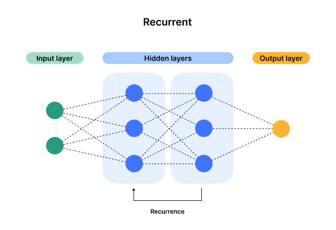
Recurrent neural networks can go backwards, allowing the output from some nodes to impact the input of preceding nodes.

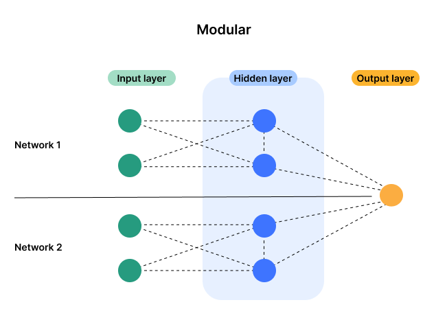
Modular neural networks combine two or more neural networks in order to arrive at the output.

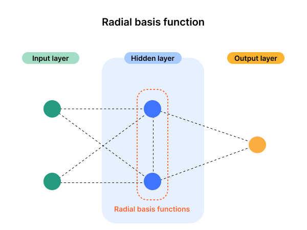
Radial basis function neural network nodes use a specific kind of mathematical function called a radial basis function.

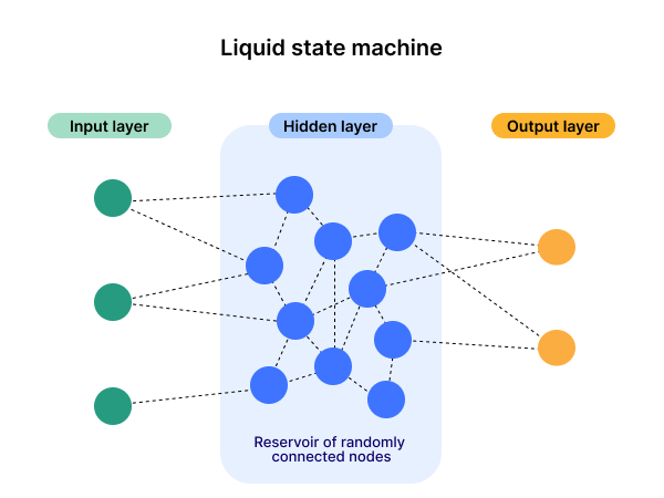
Liquid state machine neural networks feature nodes that are randomly connected to each other.

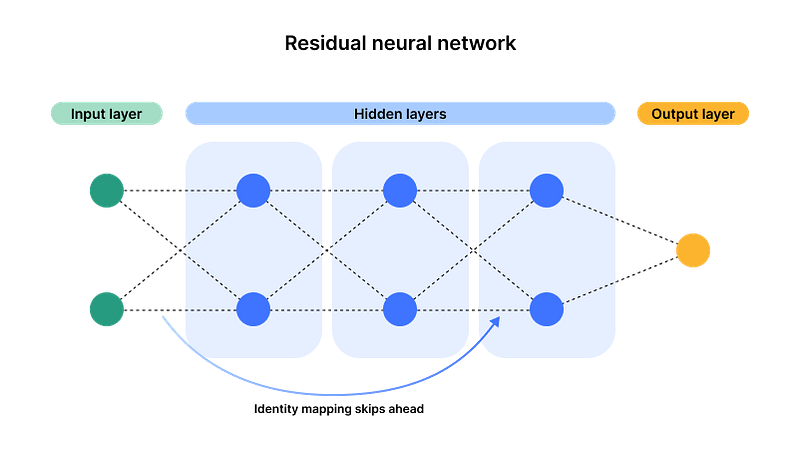
Residual neural networks allow data to skip ahead via a process called identity mapping, combining the output from early layers with the output of later layers.

This blog primarily focuses on Recurrent Neural Networks (RNNs).

2. Recurrent Neural Networks (RNNs)

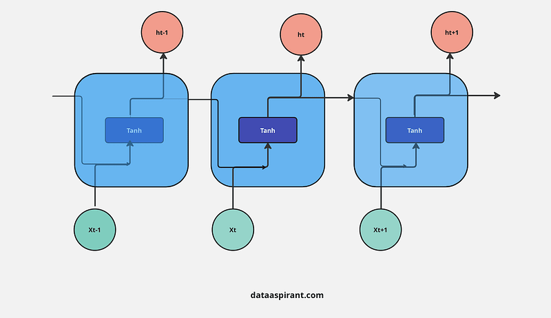
A Recurrent Neural Network (RNN) is a type of neural network architecture specifically designed to handle sequential data by maintaining a memory of previous inputs. This is achieved through connections that form loops in the network, allowing information to persist. Unlike traditional feed-forward neural networks, which assume that inputs are independent of each other, RNNs use their internal state (memory) to process sequences of inputs. This makes them especially useful for tasks where the order of inputs matters, such as time-series data, language modeling, or video sequences.

Recurrent cells are neural networks (usually small) for processing sequential data. As we already know, convolutional layers are specialized for processing grid-structured values (i.e. images). On the contrary, recurrent layers are designed for processing long sequences, without any extra sequence-based design choice.

One can achieve this by connecting the timesteps’ output to the input! This is called sequence unrolling. By processing the whole sequence, we have an algorithm that takes into account the previous states of the sequence. In this manner, we have the first notion of memory (a cell)! Let’s look at it:

The majority of common recurrent cells can also process sequences of variable length. This is really important for many applications such as videos, that contain a different number of images. One can view the RNN cell as a common neural network with shared weights for the multiple timesteps. With this modification, the weights of the cell now have access to the previous states of the sequence.

2.1 What is Sequential data?

Sequential data is information that has a specific order and where the order matters. Each piece of data in the sequence is related to the ones before and after it, and this order provides context and meaning to the data as a whole.

Here’s an example to illustrate:

Imagine a sentence like “The quick brown fox jumps over the lazy dog.” Each word in the sentence is a piece of data. The order of the words is crucial because it determines the meaning of the sentence. “Fox brown quick the jumps over lazy dog” wouldn’t make much sense, right?

Here are some other common types of sequential data:

• Time series data: This refers to data points collected at regular intervals over time. Examples include stock prices, temperature readings, or website traffic. The order of the data points matters because it shows how the value changes over time.
• Natural language text: All written language is sequential. The order of words in a sentence or paragraph is essential for conveying meaning and understanding the relationships between ideas.
• Speech signals: Spoken language is another example of sequential data. The order of sounds like phonemes, syllables, and words is crucial for understanding the spoken message.

2.2 Recurrent Neural Networks vs. Feedforward Neural Networks

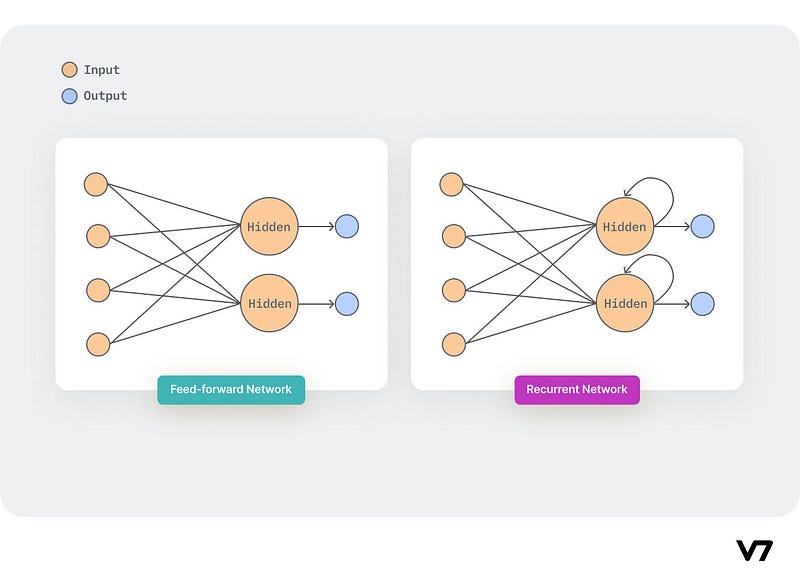
Feedforward Artificial Neural Networks allow data to flow only in one direction i.e. from input to output. The architecture of this network follows a top-down approach and has no loops i.e., the output of any layer does not affect that same layer. They are mainly used in pattern recognition.

Recurrent Neural Networks have signals traveling in both directions by using feedback loops in the network. Features derived from earlier input are fed back into the network which gives them an ability to memorize. These interactive networks are dynamic due to the ever-changing state until they reach an equilibrium point. These networks are mainly used in sequential autocorrelative data like time series.

2.3 Why use RNNs ?

1. Traditional Artificial Neural Networks (ANNs) are powerful tools, but they struggle with sequential data like text because they require fixed-size inputs. Each input in an ANN is treated independently, making them unsuitable for tasks where the order and relationships between elements are crucial.
2. Suppose we use the zero padding concept in which Shorter sequences are padded with zeros at the end to reach the length of the longest sequence in the batch. These zeros act as placeholders and don’t carry any meaningful information. Padding introduces irrelevant zeros that the network needs to process alongside the actual data, increasing the computational burden.
3. And also due to no sequences in passing input in ANN, we lose the context or sequential information. Apart from this if any user gives the input length of a higher size than we expect then in that scenario we can do nothing. For ex., we set our input size is 5 words but if any user gives it 15 words at a time then in that case we can’t handle it with ANN.

3. The Architecture of RNNs

3.1 Unfolding RNNs in Time

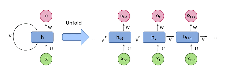
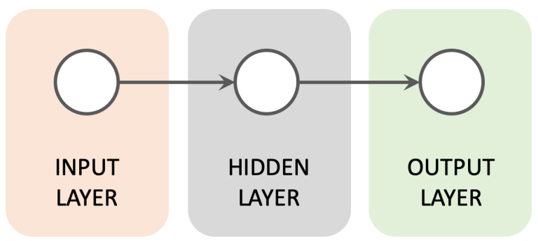
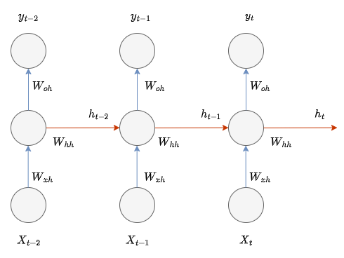
Recurrent Neural Networks differ from other neural networks mainly because they have an internal state or memory that keeps track of the data they have processed. Basically, an RNN is made up of three key components: the input layer, one or more hidden layers, and the output layer.

Input Layer This layer takes in sequences of inputs over time. Unlike feedforward networks that process all inputs at once, RNNs handle one input at a time for each time step. This sequential processing allows the network to maintain a dynamic that changes over time.

Let’s denote X_t​ as the input at time step t. This input is fed into the RNN one step at a time.

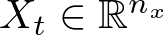
where n_x​ is the number of units (neurons) in the input layer.

For example, this is how we would initialize the input layer in Python:

self.weights_ih = np.random.randn(input_size, hidden_size) * 0.01

Here input_size is the size (number of neurons) of the input layer. hidden_size is the size of the hidden layer. self.weights_ih is the weight matrix connecting the input layer to the hidden layer, initialized with normally distributed random values, scaled by 0.01 to keep them small.

Hidden States Hidden layers are crucial in an RNN because they process not only the current input but also retain information from previous inputs. This information is stored in what we call the hidden state and is carried forward to influence future processing. This ability to carry forward information is what gives RNNs their memory capabilities.

The hidden state h_t​ at time step t is computed based on the current input Xt​ and the previous hidden state h_(t−1)​. This is expressed as:

where:

• h_t ​​ is the hidden state at time step t,
• W is the weight matrix for the hidden layer,
• b_h​ is the bias vector for the hidden layer,
• f is a nonlinear activation function, often tanh⁡tanh or ReLU.

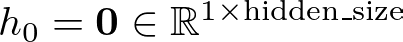
Let’s set the hidden states initially to zero: h = np.zeros((1, self.hidden_size)). This initializes the first hidden state h with zeros, preparing it for the first input in the sequence.

As the RNN processes each input in the sequence, the new hidden state is computed using both the current input x and the previous hidden state h. This happens in the loop inside the forward method, which we will build later:

for i, x in enumerate(inputs):
    x = x.reshape(1, -1)  # Ensure x is a row vector
    h = np.tanh(np.dot(x, self.weights_ih) + np.dot(h, self.weights_hh) + self.bias_h)
    self.last_hs[i + 1] = h

In each iteration of the loop, the current input x is transformed into a row vector and then multiplied by the input-to-hidden weight matrix self.weights_ih.

Simultaneously, the previous hidden state h is multiplied by the hidden-to-hidden weight matrix self.weights_hh. The results of these two operations are summed with the hidden bias self.bias_h.

The sum is then passed through the np.tanh function, which applies a nonlinear transformation and yields the new hidden state h for the current timestep.

This new hidden state h is stored in a dictionary self.last_hs with the current timestep as the key. This allows the network to "remember" the hidden states at each step, which is essential for the backpropagation through time (BPTT) during training.

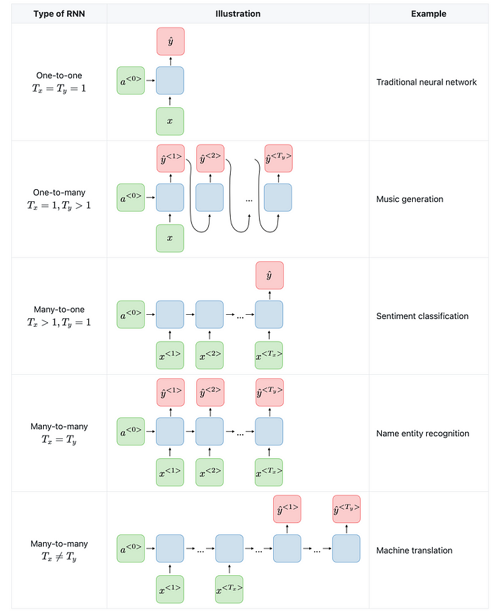
Output Sequences RNNs are flexible in how they output results. They can output at each timestep (many-to-many), produce a single output at the end of a sequence (many-to-one), or even generate a sequence from a single input (one-to-many). This flexibility makes RNNs useful for a range of tasks like language modeling and time-series analysis.

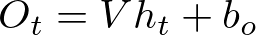
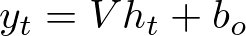
The output at each time step O_t​ can be calculated from the hidden state. For a many-to-many RNN:

​where:

• O_t​​ is the output at time step t,
• V is the weight matrix for the output layer,
• b_o is the bias vector for the output layer.

For a many-to-one RNN, you would only compute the output at the final time step, while for a one-to-many RNN, you would start with a single input to generate a sequence of outputs.

The computed output Ot​ is often passed through a softmax function if the RNN is used for classification tasks to obtain probabilities of different classes.

where P(y_t​ ∣ X_t​, h_(t−1​)) is the probability of the output yt​ given the input Xt​ and the previously hidden state h_(t−1​).

The sequence of operations from input to hidden state to output captures the essence of RNNs’ ability to maintain and utilize temporal information, allowing them to perform complex tasks that involve sequences and time.

RNNs have a loop within them that allows information to flow from a later stage of the model back to an earlier stage. This looping mechanism is what enables them to process sequences of data: it allows outputs from the network to influence subsequent inputs processed by the same network. This fundamental difference is what enables RNNs to perform tasks that involve sequences and time-series data effectively.

3.2 Key Operations in RNNs

Understanding how Recurrent Neural Networks (RNNs) operate is essential for using them effectively and improving their performance. Let’s break down the main operations within an RNN:

3.2.1 Forward Pass

In the forward pass, an RNN processes data one step at a time. For each timestep, it combines the current input with the previous hidden state to compute the new hidden state and the output. The model use specific functions that are inherently recurrent, meaning each output depends on the preceding computations. Functions like the sigmoid or tanh are commonly used to introduce non-linearity, helping to manage how information is transformed within the hidden layers.

Here’s how the math plays out:

Initially, we set the hidden state h to a vector of zeros. This is represented mathematically as:

Or in Python terms:

h = np.zeros((1, self.hidden_size))

As we move through each input in the sequence, we compute the new hidden state at time step t, denoted h_t​, based on the previous hidden state h_(t−1)​, the current input x_t​, and the associated weights and biases:

where we can define U, W, and b_h as:

self.weights_ih = np.random.randn(input_size, hidden_size) * 0.01
self.weights_hh = np.random.randn(hidden_size, hidden_size) * 0.01
self.weights_ho = np.random.randn(hidden_size, output_size) * 0.01

Here:

• U is self.weights_ih, the weight matrix connecting inputs to the hidden layer.
• W is self.weights_hh, the weight matrix connecting the hidden layer at one timestep to the next.
• b_h​ is self.bias_h, the bias term for the hidden layer.
• tanh represents the hyperbolic tangent function, introducing non-linearity into the equation.

This mirrors the loop in the forward method that iterates over each input.

The output at time step t, which we call y_t​, is then calculated from the hidden state using another set of weights and biases:

​In this case:

• V is self.weights_ho, the weight matrix from the hidden layer to the output layer.
• b_o​ is self.bias_o, the output layer bias.

The code y = np.dot(h, self.weights_ho) + self.bias_o corresponds to this equation, which generates the output based on the hidden state at the final timestep.

3.2.2 Backpropagation Through Time (BPTT)

Training RNNs involves a special kind of backpropagation called BPTT. Unlike traditional backpropagation, BPTT extends across time — it unfolds the entire sequence of data, applying backpropagation at each timestep. This method calculates gradients for each output, which are then used to adjust the weights and reduce the overall loss. However, BPTT can be complex and resource-intensive, and it’s prone to issues such as vanishing and exploding gradients, which can interfere with the network’s ability to learn from data over longer sequences.

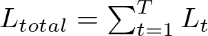
Given a sequence of T timesteps and assuming a simple loss function L at each timestep t, such as mean squared error for regression tasks or categorical cross-entropy for classification tasks, the total loss L_total​ is the sum of the losses at each timestep:

​To update the weights, we need to calculate the gradient of L_total​ with respect to the weights. For the weight matrices U (input to hidden), W (hidden to hidden), and V (hidden to output), we have:

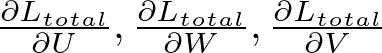
​​These gradients are computed using the chain rule. Starting from the final timestep and moving backwards:

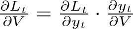
Where:

• ​∂L_t/∂y_t​​ is the derivative of the loss function at timestep t with respect to the output y_t​.
• ∂y_t/∂V​​ can be directly calculated as the hidden state h_t​ because y_t​ = V_h_t​ + b_o​.

For W and U, the calculation involves the recurrent nature of the network:

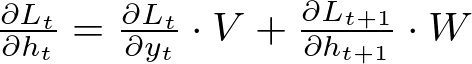
Here, ​∂Lt+1​ / ∂ht+1​ refers to the gradient of the loss at timestep t+1 with respect to the hidden state at t+1, which in turn depends on the hidden state at t. This recurrence relation forms the crux of BPTT.

3.2.3 Weight Updates

With the gradients calculated, the weights are updated using an optimization algorithm such as stochastic gradient descent (SGD):

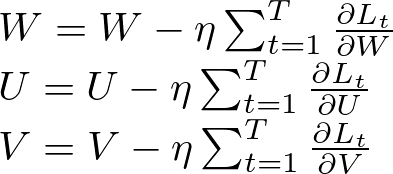
​​Where η is the learning rate.

4. Challenges in Training RNNs

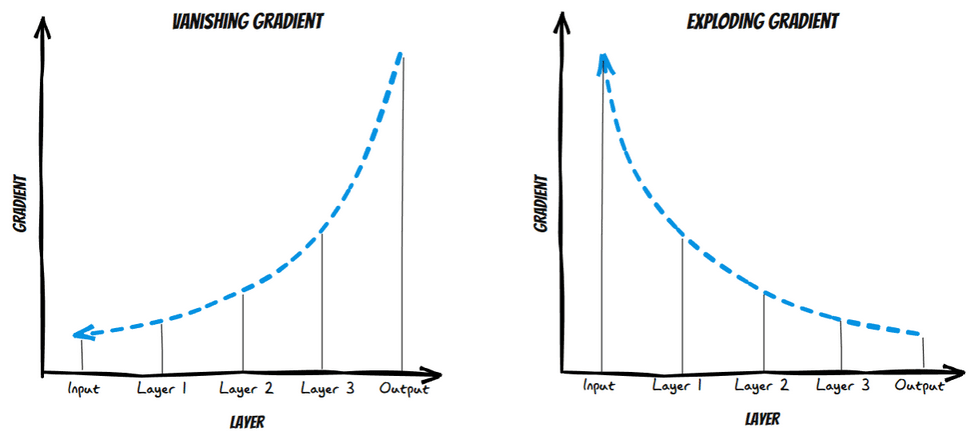
4.1 What is Vanishing Gradient?

As the backpropagation algorithm advances downwards(or backward) from the output layer towards the input layer, the gradients often get smaller and smaller and approach zero which eventually leaves the weights of the initial or lower layers nearly unchanged. As a result, the gradient descent never converges to the optimum. This is known as the vanishing gradients problem.

4.2 What is Exploding Gradient?

On the contrary, in some cases, the gradients keep on getting larger and larger as the backpropagation algorithm progresses. This, in turn, causes very large weight updates and causes the gradient descent to diverge. This is known as the exploding gradients problems.

4.3 Why Do the Gradients Even Vanish/Explode?

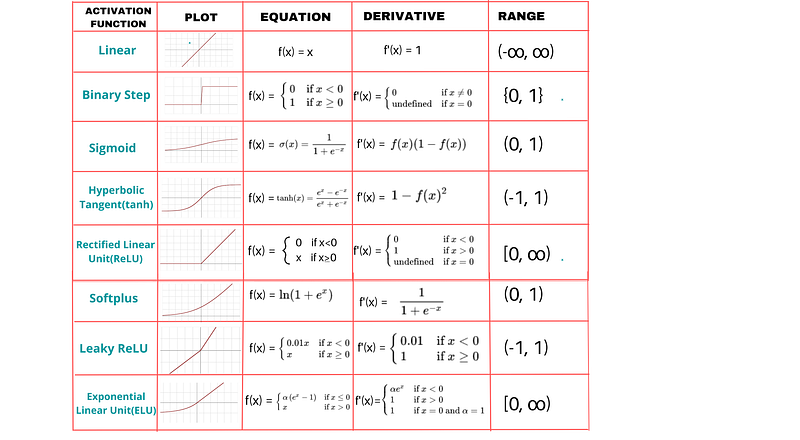
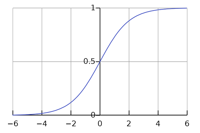
Certain activation functions, like the logistic function (sigmoid), have a very huge difference between the variance of their inputs and the outputs. In simpler words, they shrink and transform a larger input space into a smaller output space that lies between the range of [0,1].

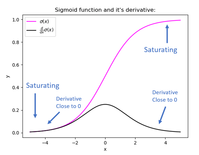
Observing the above graph of the Sigmoid function, we can see that for larger inputs (negative or positive), it saturates at 0 or 1 with a derivative very close to zero. Thus, when the backpropagation algorithm chips in, it virtually has no gradients to propagate backward in the network, and whatever little residual gradients exist keeps on diluting as the algorithm progresses down through the top layers. So, this leaves nothing for the lower layers.

Similarly, in some cases suppose the initial weights assigned to the network generate some large loss. Now the gradients can accumulate during an update and result in very large gradients which eventually results in large updates to the network weights and leads to an unstable network. The parameters can sometimes become so large that they overflow and result in NaN values.

4.4 How to Know if Our Model is Suffering From the Exploding/Vanishing Gradient Problem?

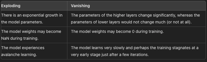
Following are some signs that can indicate that our gradients are vanishing and exploding gradients :

Certainly, neither do we want our signal to explode or saturate nor do we want it to die out. The signal needs to flow properly both in the forward direction when making predictions as well as in the backward direction while calculating gradients.

5. Handle Vanishing/Exploding Gradients

Now that we understand the vanishing/exploding gradients problems, we can learn some techniques to fix them.

5.1 Proper Weight Initialization

Researchers Xavier Glorot, Antoine Bordes, and Yoshua Bengio proposed a way to remarkably alleviate this problem.

For the proper flow of the signal, the authors argue that:

• The variance of outputs of each layer should be equal to the variance of its inputs.
• The gradients should have equal variance before and after flowing through a layer in the reverse direction.

Although both conditions cannot hold for any layer in the network unless the number of inputs to the layer (fanin) equals the number of neurons in the layer (fanout), they proposed a well-proven compromise that works incredibly well in practice. They randomly initialize the connection weights for each layer in the network using the following equation, popularly known as Xavier initialization (after the author’s first name) or Glorot initialization (after his last name).

where  fanavg = ( fanin + fanout ) / 2

• Normal distribution with mean 0 and variance σ2 = 1/ fanavg
• Or a uniform distribution between -r and +r , with r = sqrt( 3 / fanavg )

Following are some more very popular weight initialization strategies for different activation functions, they only differ by the scale of variance and by the usage of either fanavg or fanin

for uniform distribution, calculate r as: r = sqrt( 3*σ2 )

Using the above initialization strategies can significantly speed up the training and increase the odds of gradient descent converging at a lower generalization error.

Wait, but how do we put these strategies into code ??

Relax! we will not need to hardcode anything, Keras does it for us.

• Keras uses Xavier’s initialization strategy with uniform distribution.
• If we wish to use a different strategy than the default one, this can be done using the kernel_initializer parameter while creating the layer. For example :

keras.layer.Dense(25, activation = "relu", kernel_initializer="he_normal")

or

keras.layer.Dense(25, activation = "relu", kernel_initializer="he_uniform")

If we wish to use use the initialization based on fanavg rather than fanin , we can use the VarianceScaling initializer like this :

he_avg_init = keras.initializers.VarianceScaling(scale=2., mode='fan_avg', distribution='uniform')
keras.layers.Dense(20, activation="sigmoid", kernel_initializer=he_avg_init)

5.2 Using Non-saturating Activation Functions

In an earlier section, while studying the nature of sigmoid activation function, we observed that its nature of saturating for larger inputs (negative or positive) came out to be a major reason behind the vanishing and exploding gradients thus making it non-recommendable to use in the hidden layers of the network.

So to tackle the issue regarding the saturation of activation functions like sigmoid and tanh, we must use some other non-saturating functions like ReLu and its alternatives.

ReLU ( Rectified Linear Unit )

Relu(z) = max(0,z)

• Outputs 0 for any negative input.
• Range: [0, infinity]

Unfortunately, the ReLu function is also not a perfect pick for the intermediate layers of the network “in some cases”. It suffers from a problem known as dying ReLus wherein some neurons just die out, meaning they keep on throwing 0 as outputs with the advancement in training.

Read about the dying relus problem in detail here.

Some popular alternative functions of the ReLU that mitigates the problem of vanishing gradients when used as activation for the intermediate layers of the network are LReLU, PReLU, ELU, SELU :

LReLU (Leaky ReLU)

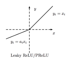
LeakyReLUα(z) = max(αz, z)

• The amount of “leak” is controlled by the hyperparameter α, it is the slope of the function for z < 0.
• The smaller slope for the leak ensures that the neurons powered by leaky Relu never die; although they might venture into a state of coma for a long training phase they always have a chance to eventually wake up.
• The model can also train α, learning its value during training. This variant, where α is considered a parameter rather than a hyperparameter, is called parametric leaky ReLU (PReLU).

ELU (Exponential Linear Unit)

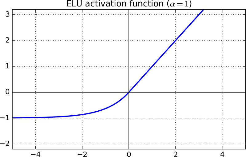
For z < 0, it takes on negative values which allow the unit to have an average output closer to 0 thus alleviating the vanishing gradient problem

• For z < 0, the gradients are non zero. This avoids the dead neurons problem.
• For α = 1, the function is smooth everywhere, this speeds up the gradient descent since it does not bounce right and left around z=0.
• A scaled version of this function ( SELU: Scaled ELU ) is also used very often in Deep Learning.

5.3 Batch Normalization

Using He initialization along with any variant of the ReLU activation function can significantly reduce the chances of vanishing/exploding problems at the beginning. However, it does not guarantee that the problem won’t reappear during training.

In 2015, Sergey Ioffe and Christian Szegedy proposed a paper in which they introduced a technique known as Batch Normalization to address the problem of vanishing/exploding gradient problem.

The Following key points explain the intuition behind BN and how it works:

• It consists of adding an operation in the model just before or after the activation function of each hidden layer.
• This operation simply zero-centers and normalizes each input, then scales and shifts the result using two new parameter vectors per layer: one for scaling, the other for shifting.
• In other words, the operation lets the model learn the optimal scale and mean of each of the layer’s inputs.
• To zero-center and normalize the inputs, the algorithm needs to estimate each input’s mean and standard deviation.
• It does so by evaluating the mean and standard deviation of the input over the current mini-batch (hence the name “Batch Normalization”).

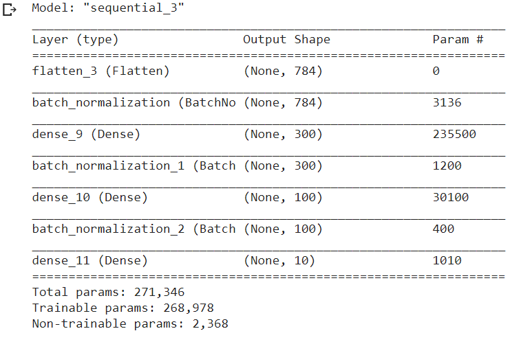
model = keras.models.Sequential([keras.layers.Flatten(input_shape=[28, 28]),keras.layers.BatchNormalization(),keras.layers.Dense(300, activation="relu"),keras.layers.BatchNormalization(),keras.layers.Dense(100, activation="relu"),keras.layers.BatchNormalization(),keras.layers.Dense(10, activation="softmax")])

we just added batch normalization after each layer ( dataset : FMNIST)

model.summary()

5.4 Gradient Clipping

Another popular technique to mitigate the exploding gradient problem is to clip the gradients during backpropagation so that they never exceed some threshold. This is called Gradient Clipping.

• This optimizer will clip every component of the gradient vector to a value between –1.0 and 1.0.
• This means we will clip all the partial derivatives of the loss with respect to each trainable parameter between –1.0 and 1.0.

optimizer = keras.optimizers.SGD(clipvalue = 1.0)

• The threshold is a hyperparameter we can tune.
• The orientation of the gradient vector may change due to this: for eg, let the original gradient vector be [0.9, 100.0] pointing mostly in the direction of the second axis, but once we clip it by some value, we get [0.9, 1.0] which now points somewhere around the diagonal between the two axes.
• To ensure that the orientation remains intact even after clipping, we should clip by norm rather than by value.

optimizer = keras.optimizers.SGD(clipnorm = 1.0)

• If the threshold we pick is less than the ℓ2 norm, we will clip the whole gradient. For example, if clipnorm=1, we will clip the vector [0.9, 100.0] to [0.00899, 0.999995], thus preserving its orientation.

6. Building RNN from Scratch

For this demonstration, we will use the Air passenger dataset, which is a small open-source dataset hosted on GitHub.

Let’s dive into the details of each component in the code to create a comprehensive guide on how this RNN is implemented from scratch!

6. 1 Defining the RNN Class

import numpy as np
import pandas as pd
import matplotlib.pyplot as plt

class RNN:
    def __init__(self, input_size, hidden_size, output_size, init_method="random"):
        self.weights_ih, self.weights_hh, self.weights_ho = self.initialize_weights(input_size, hidden_size, output_size, init_method)
        self.bias_h = np.zeros((1, hidden_size))
        self.bias_o = np.zeros((1, output_size))
        self.hidden_size = hidden_size

    def initialize_weights(self, input_size, hidden_size, output_size, method):
        if method == "random":
            weights_ih = np.random.randn(input_size, hidden_size) * 0.01
            weights_hh = np.random.randn(hidden_size, hidden_size) * 0.01
            weights_ho = np.random.randn(hidden_size, output_size) * 0.01
        elif method == "xavier":
            weights_ih = np.random.randn(input_size, hidden_size) / np.sqrt(input_size / 2)
            weights_hh = np.random.randn(hidden_size, hidden_size) / np.sqrt(hidden_size / 2)
            weights_ho = np.random.randn(hidden_size, output_size) / np.sqrt(hidden_size / 2)
        elif method == "he":
            weights_ih = np.random.randn(input_size, hidden_size) * np.sqrt(2 / input_size)
            weights_hh = np.random.randn(hidden_size, hidden_size) * np.sqrt(2 / hidden_size)
            weights_ho = np.random.randn(hidden_size, output_size) * np.sqrt(2 / hidden_size)
        else:
            raise ValueError("Invalid initialization method")
        return weights_ih, weights_hh, weights_ho


    def forward(self, inputs):
        h = np.zeros((1, self.hidden_size))
        self.last_inputs = inputs
        self.last_hs = {0: h}

        for i, x in enumerate(inputs):
            x = x.reshape(1, -1)  # Ensure x is a row vector
            h = np.tanh(np.dot(x, self.weights_ih) + np.dot(h, self.weights_hh) + self.bias_h)
            self.last_hs[i + 1] = h

        y = np.dot(h, self.weights_ho) + self.bias_o
        self.last_outputs = y
        return y

    def backprop(self, d_y, learning_rate, clip_value=1):
        n = len(self.last_inputs)

        d_y_pred = (self.last_outputs - d_y) / d_y.size
        d_Whh = np.zeros_like(self.weights_hh)
        d_Wxh = np.zeros_like(self.weights_ih)
        d_Why = np.zeros_like(self.weights_ho)
        d_bh = np.zeros_like(self.bias_h)
        d_by = np.zeros_like(self.bias_o)
        d_h = np.dot(d_y_pred, self.weights_ho.T)

        for t in reversed(range(1, n + 1)):
            d_h_raw = (1 - self.last_hs[t] ** 2) * d_h
            d_bh += d_h_raw
            d_Whh += np.dot(self.last_hs[t - 1].T, d_h_raw)
            d_Wxh += np.dot(self.last_inputs[t - 1].reshape(1, -1).T, d_h_raw)
            d_h = np.dot(d_h_raw, self.weights_hh.T)

        for d in [d_Wxh, d_Whh, d_Why, d_bh, d_by]:
            np.clip(d, -clip_value, clip_value, out=d)
            
        self.weights_ih -= learning_rate * d_Wxh
        self.weights_hh -= learning_rate * d_Whh
        self.weights_ho -= learning_rate * d_Why
        self.bias_h -= learning_rate * d_bh
        self.bias_o -= learning_rate * d_by

This is the blueprint for our RNN.

We will define the RNN’s initialization, forward pass, and backpropagation within this class.

RNN Initialization

class RNN:
  def __init__(self, input_size, hidden_size, output_size, init_method="random"):
    self.weights_ih, self.weights_hh, self.weights_ho = self.initialize_weights(input_size, hidden_size, output_size, init_method)
    self.bias_h = np.zeros((1, hidden_size))
    self.bias_o = np.zeros((1, output_size))
    self.hidden_size = hidden_size

The __init__ method initializes the RNN with the number of neurons in each layer (input, hidden, output) and the method for weight initialization.

self.weights_ih, self.weights_hh, self.weights_ho = self.initialize_weights(input_size, hidden_size, output_size, init_method)

Here we call the initialize_weights method to set the weights according to the specified initialization method—'random', 'xavier', or 'he'. Each set of weights connects different layers of the network: weights_ih connects the input layer to the hidden layer, weights_hh connects the hidden layer to itself at the next timestep (capturing the 'recurrent' part of the RNN), and weights_ho connects the hidden layer to the output layer.

self.bias_h = np.zeros((1, hidden_size))
self.bias_o = np.zeros((1, output_size))

Biases are initialized to zero vectors, which will be adjusted during training. There’s one bias for the hidden layer and one for the output layer.

Forward Pass Method

def forward(self, inputs):
    h = np.zeros((1, self.hidden_size))
    self.last_inputs = inputs
    self.last_hs = {0: h}
  
    for i, x in enumerate(inputs):
        x = x.reshape(1, -1)  # Ensure x is a row vector
        h = np.tanh(np.dot(x, self.weights_ih) + np.dot(h, self.weights_hh) + self.bias_h)
        self.last_hs[i + 1] = h
  
    y = np.dot(h, self.weights_ho) + self.bias_o
    self.last_outputs = y
    return y

The forward function takes a sequence of inputs and processes it through the RNN. It computes the hidden states and the final output in a loop over the sequence length.

h = np.zeros((1, self.hidden_size))

This initializes the hidden state as a vector of zeros. As the network sees more of the input sequence, this state will be updated to capture information from the inputs.

for i, x in enumerate(inputs):
    x = x.reshape(1, -1)  # Ensure x is a row vector
    h = np.tanh(np.dot(x, self.weights_ih) + np.dot(h, self.weights_hh) + self.bias_h)
    self.last_hs[i + 1] = h

For each input in the sequence, the code reshapes the input to ensure it’s a row vector, then updates the hidden state using the current input, previous hidden state, weights, and biases. The np.tanh function introduces non-linearity necessary for complex pattern recognition.

y = np.dot(h, self.weights_ho) + self.bias_o

After processing the entire sequence, we compute the output using the last hidden state, the weights connecting the hidden layer to the output layer, and the output bias.

Backpropagation Through Time

def backprop(self, d_y, learning_rate, clip_value=1):
    n = len(self.last_inputs)
  
    d_y_pred = (self.last_outputs - d_y) / d_y.size
    d_Whh = np.zeros_like(self.weights_hh)
    d_Wxh = np.zeros_like(self.weights_ih)
    d_Why = np.zeros_like(self.weights_ho)
    d_bh = np.zeros_like(self.bias_h)
    d_by = np.zeros_like(self.bias_o)
    d_h = np.dot(d_y_pred, self.weights_ho.T)
  
    for t in reversed(range(1, n + 1)):
        d_h_raw = (1 - self.last_hs[t] ** 2) * d_h
        d_bh += d_h_raw
        d_Whh += np.dot(self.last_hs[t - 1].T, d_h_raw)
        d_Wxh += np.dot(self.last_inputs[t - 1].reshape(1, -1).T, d_h_raw)
        d_h = np.dot(d_h_raw, self.weights_hh.T)
  
    for d in [d_Wxh, d_Whh, d_Why, d_bh, d_by]:
        np.clip(d, -clip_value, clip_value, out=d)
        
    self.weights_ih -= learning_rate * d_Wxh
    self.weights_hh -= learning_rate * d_Whh
    self.weights_ho -= learning_rate * d_Why
    self.bias_h -= learning_rate * d_bh
    self.bias_o -= learning_rate * d_by

The backprop method implements the BPTT algorithm. It calculates gradients for each timestep and updates the weights and biases accordingly. Additionally, it incorporates gradient clipping by using np.clip to prevent the exploding gradients problem.

6.2 Early Stopping Mechanism

class EarlyStopping:
   def __init__(self, patience=7, verbose=False, delta=0):
        self.patience = patience
        self.verbose = verbose
        self.counter = 0
        self.best_score = None
        self.early_stop = False
        self.delta = delta

    def __call__(self, val_loss):
        score = -val_loss

        if self.best_score is None:
            self.best_score = score

        elif score < self.best_score + self.delta:
            self.counter += 1
            
            if self.counter >= self.patience:
                self.early_stop = True
        else:
            self.best_score = score
            self.counter = 0

This class provides an early stopping mechanism during training. If the validation loss hasn’t improved after a certain number of epochs (patience), training is halted to prevent overfitting.

I won’t dive into this class’ explanation as I explained in detail in this previous article:

6.3 RNN Trainer Class

class RNNTrainer:
    def __init__(self, model, loss_func='mse'):
        self.model = model
        self.loss_func = loss_func
        self.train_loss = []
        self.val_loss = []

    def calculate_loss(self, y_true, y_pred):
        if self.loss_func == 'mse':
            return np.mean((y_pred - y_true)**2)
        
        elif self.loss_func == 'log_loss':
            return -np.mean(y_true*np.log(y_pred) + (1-y_true)*np.log(1-y_pred))
        
        elif self.loss_func == 'categorical_crossentropy':
            return -np.mean(y_true*np.log(y_pred))
        
        else:
            raise ValueError('Invalid loss function')

    def train(self, train_data, train_labels, val_data, val_labels, epochs, learning_rate, early_stopping=True, patience=10, clip_value=1):
        if early_stopping:
            early_stopping = EarlyStopping(patience=patience, verbose=True)
        for epoch in range(epochs):
            for X_train, y_train in zip(train_data, train_labels):
                outputs = self.model.forward(X_train)
                self.model.backprop(y_train, learning_rate, clip_value)
                train_loss = self.calculate_loss(y_train, outputs)
                self.train_loss.append(train_loss)

            val_loss_epoch = []
            for X_val, y_val in zip(val_data, val_labels):
                val_outputs = self.model.forward(X_val)
                val_loss = self.calculate_loss(y_val, val_outputs)
                val_loss_epoch.append(val_loss)

            val_loss = np.mean(val_loss_epoch)
            self.val_loss.append(val_loss)

            if early_stopping:
                early_stopping(val_loss)

                if early_stopping.early_stop:
                    print(f"Early stopping at epoch {epoch} | Best validation loss = {-early_stopping.best_score:.3f}")
                    break

            if epoch % 10 == 0:
                print(f'Epoch {epoch}: Train loss = {train_loss:.4f}, Validation loss = {val_loss:.4f}')

    def plot_gradients(self):
        for i, gradients in enumerate(zip(*self.gradients)):
            plt.plot(gradients, label=f'Neuron {i}')

        plt.xlabel('Time step')
        plt.ylabel('Gradient')
        plt.title('Gradients for each neuron over time')
        plt.legend()
        plt.show()

This class wraps up the training process. It takes care of running the forward pass and backpropagation, computes the loss after each epoch, and maintains a history of training and validation losses.

Training Method

Above we define the method that will train the RNN model. It loops over the specified number of epochs, processes the training data through the model, applies backpropagation, and tracks the training and validation losses.

6.4 Data Loading and Preprocessing

class TimeSeriesDataset:
    def __init__(self, url, look_back=1, train_size=0.67):
        self.url = url
        self.look_back = look_back
        self.train_size = train_size

    def load_data(self):
        df = pd.read_csv(self.url, usecols=[1])
        df = self.MinMaxScaler(df.values)  # Convert DataFrame to numpy array
        train_size = int(len(df) * self.train_size)
        train, test = df[0:train_size,:], df[train_size:len(df),:]
        return train, test
    
    def MinMaxScaler(self, data):
        numerator = data - np.min(data, 0)
        denominator = np.max(data, 0) - np.min(data, 0)
        return numerator / (denominator + 1e-7)

    def create_dataset(self, dataset):
        dataX, dataY = [], []
        for i in range(len(dataset)-self.look_back-1):
            a = dataset[i:(i+self.look_back), 0]
            dataX.append(a)
            dataY.append(dataset[i + self.look_back, 0])
        return np.array(dataX), np.array(dataY)

    def get_train_test(self):
        train, test = self.load_data()
        trainX, trainY = self.create_dataset(train)
        testX, testY = self.create_dataset(test)
        return trainX, trainY, testX, testY

This class handles the loading, preprocessing, and batching of time-series data. It is designed to facilitate the handling of data that will be fed into the RNN.

def load_data(self): Loads data from a CSV file specified by a URL. It uses Pandas to handle the CSV and extracts the necessary columns.

def MinMaxScaler(self, data): This is a normalization function that scales the data between 0 and 1. This is a common practice in time series and other types of data processing to help neural networks learn more effectively.

def create_dataset(self, dataset): It reformats the loaded data into a suitable format where dataX contains input sequences for the model and dataY contains the corresponding labels or targets for each sequence.

def get_train_test(self): This splits the loaded data into training and testing datasets based on a specified proportion.

Loading and Preparing the Data

url = 'https://raw.githubusercontent.com/jbrownlee/Datasets/master/daily-min-temperatures.csv'
dataset = TimeSeriesDataset(url, look_back=1)
trainX, trainY, testX, testY = dataset.get_train_test()

Here, we specify the URL of the dataset, instantiate the TimeSeriesDataset with a look_back of 1, which means each input sequence (used for training the RNN) will consist of 1 timestep. The data is then split into training and testing sets.

trainX = np.reshape(trainX, (trainX.shape[0], 1, trainX.shape[1]))
testX = np.reshape(testX, (testX.shape[0], 1, testX.shape[1]))

The input data needs to be reshaped to fit the RNN input requirements, which generally expect data in the format of [samples, time steps, features].

6.5 Training the RNN

rnn = RNN(look_back, 256, 1, init_method='xavier')
trainer = RNNTrainer(rnn, 'mse')
trainer.train(trainX, trainY, testX, testY, epochs=100, learning_rate=0.01, early_stopping=True, patience=10, clip_value=1)

The RNN model is instantiated with Xavier initialization, and then it is trained using the RNNTrainer. The trainer uses Mean Squared Error ('mse') as the loss function, which is suitable for regression tasks like time-series forecasting.

This implementation covers all the basic components needed to set up, train, and use an RNN for a simple time-series prediction task. The code structure facilitates understanding and modification for more complex or different types of sequence modeling tasks.

7. Long Short-Term Memory Networks (LSTMs)

In our above discussion on Recurrent Neural Networks (RNNs), we looked at how their design lets them process sequences effectively. This makes them perfect for tasks where the sequence and context of data matter, like analyzing time-series data or processing language.

Now, we’re moving on to a type of RNN that tackles one of the big challenges traditional RNNs face: managing long-term data dependencies. These are the Long Short-Term Memory Networks (LSTMs), which are a step up in complexity. They use a system of gates that control how information flows through the network — deciding what to keep and what to forget over extended sequences.

LSTM(Long-Short-Term-Memory) is one of the family or a special kind of recurrent neural network (RNN). LSTM can be a default behaviour to learn long-term dependencies by remembering essential and relevant information for a long time.

Let’s break down the core idea behind LSTMs with a simple story:

Once, King Vikram defeated King XYZ but passed away. His son, Vikram Junior, took over, fought bravely, but also died in battle. Vikram Super Junior, his grandson, wasn’t as strong but used his intelligence to finally defeat King XYZ, avenging his family.

When reading this story or any sequence of events, our minds first focus on the immediate details. For example, we process King Vikram’s victory and death. But as more characters are introduced, we adjust our long-term understanding of the story, keeping track of Vikram Junior and Super Junior. This constant updating of context mirrors how LSTMs work: they maintain and update both short-term and long-term memory as new information flows in.

RNNs struggle to balance short- and long-term context. Just like how we vividly remember the latest episode of a show but forget earlier details, RNNs often lose long-term information as new data arrives. LSTMs address this by creating two pathways — one for short-term memory and one for long-term memory — allowing the model to retain essential information and discard what’s less important.

In LSTMs, information flows through cell states, which act like a conveyor belt, carrying useful information forward while selectively forgetting irrelevant details. Unlike RNNs, where new data overwrites old data, LSTMs apply careful mathematical operations — addition and multiplication — to preserve critical information. This allows them to effectively prioritize and manage both new and past data.

Every cell state depends on three different dependencies. There are:

1. Previous cell state (the information which one is stored at the end of the previous time step)
2. Previous hidden state ( same as the output of the previous cell)
3. Input at the current time step (the new information/input at the present time step).

Having said that, let’s discuss the architecture and functionalities of the LSTM in more detail.

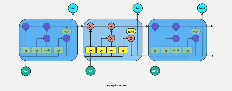
8. LSTM Architecture

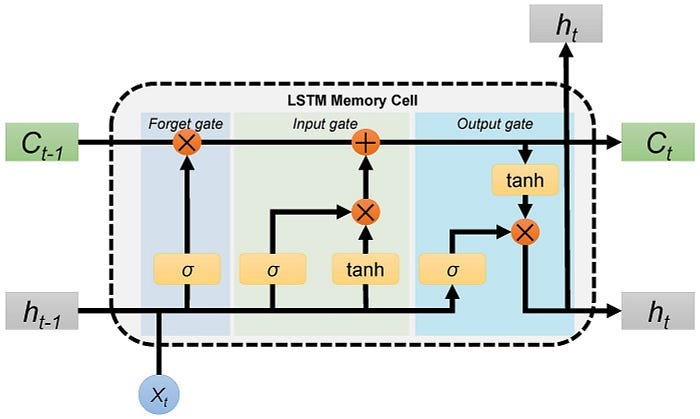
Recurrent Neural Networks (RNNs) architecture has a chain of repeating neural networks. This repeating module has a simple and single function: the tanh activation function.

LSTM architecture is also the same as the RNNs, a chain of repeating modules/neural networks. But instead of having only one tanh layer, LSTM repeating models have four different functions.

These four functional operations are especially connected. There are

• Sigmoid Activation Function
• Tanh Activation Function
• Pointwise Multiplication
• Pointwise Addition

In the whole network, information is transferred in a vector form. Let’s discuss the different signs mentioned in the above diagram:

• Square Box: a single neural network
• Circle: pointwise operation means the operation is performed element by element
• Arrow Mark: vector information is transformed from one layer to another layer
• Joining two lines into one line: concatenate two vectors
• Splitting one line into two lines: transferring the same information into two different operations or layers.

First, let’s discuss the main functions and operations in the LSTM architecture.

8.1 Activation Functions and Linear Operations

Sigmoid Function

The sigmoid function is also known as the logistic activation function. This function has a smooth and ‘S’ shape curve.

The output results of a sigmoid are always in the range of 0 and 1.

The sigmoid activation function is mainly used for models where we must predict the probabilities as outputs. Since the probability of any input exists only between the range of 0 and 1, the sigmoid or logistic activation function is the right and best choice.

Tanh Activation Function

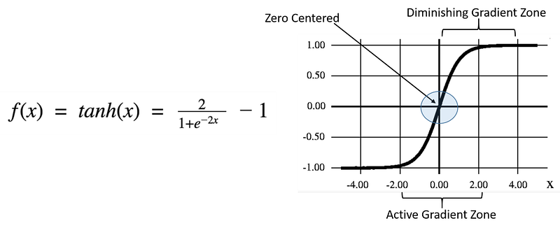
Tanh activation function also looks similar to the sigmoid/logistic function. Actually, it is a scaled sigmoid function. We can write the tanh function formula as a sigmoid function.

The range of tanh function result values are -1 to +1. Using this tanh function, we can find strongly positive, neutral, or negative input.

Pointwise Multiplication

Pointwise multiplication of two vectors is applying multiplication operations on both vectors of individual elements. For example

• A = [1,2,3,4]
• B = [2,3,4,5]
• Pointwise multiplication result : [2,6,12,20]

Pointwise Addition

Pointwise addition of two vectors is the process of adding two vector elements individually. For example

• A = [1,2,3,4]
• B = [2,3,4,5]
• Pointwise addition result : [3,5,7,9]

8.2 The Key Concepts Behind the LSTM Algorithm

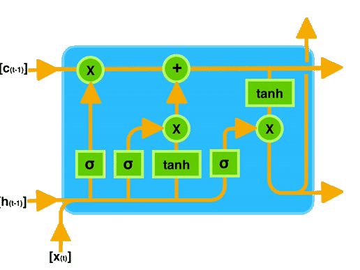
The primary unique behaviour of an LSTM is the cell state; it acts as the conveyor belt with some minor linear interactions.

This means this cell state moves the information with basic operations like addition and multiplication; that’s why information smoothly flows along with the cell state without too many changes compared to their original one.

Cell state or a conveyor belt of LSTM is the highlighted horizontal line in the below image.

LSTMs have unique structures to identify which information is essential or not important. LSTMs can remove or add information to the cell state based on importance. These special kinds of structures are called gates.

Gates are a unique way to transform information, and LSTMs use these gates to decide which information is to remember, remove, and pass to another layer, etc.

LSTM will remove or add information to the conveyor belt(cell state) based on this information. Every gate comprises a sigmoid neural net layer and a pointwise multiplication operation.

LSTMs have three kinds of gates. There are

• Forget Gate
• Input Gate
• Output Gate

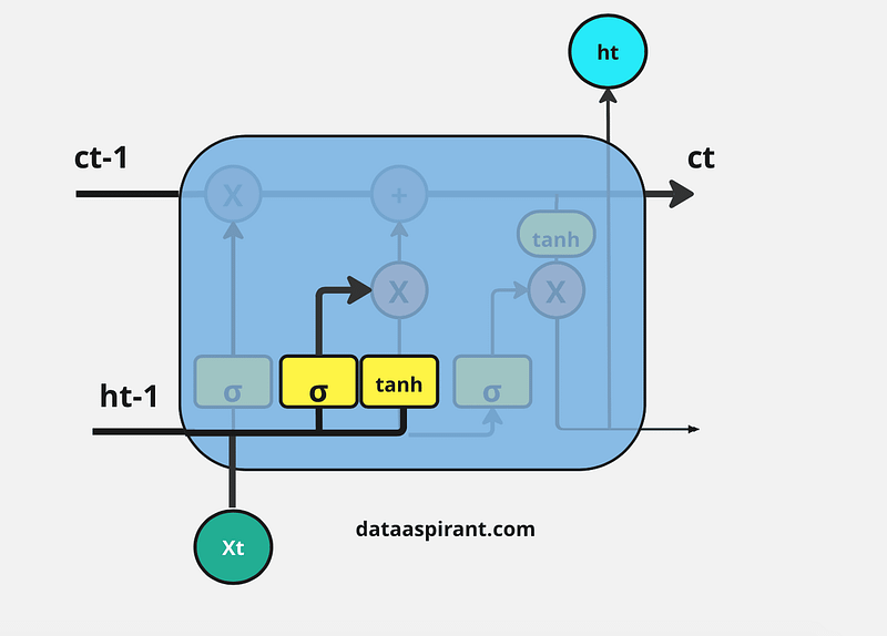
8.2.1 Forget Gate

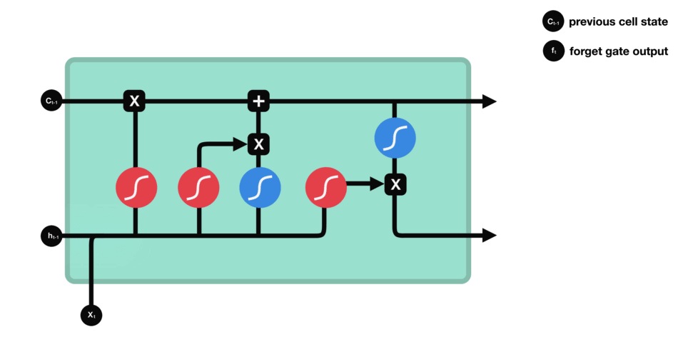
In the repeating module of the LSTM architecture, the first gate we have is the forget gate. This gate’s primary task is to decide which information should be kept or thrown away.

This means deciding which information to send to the cell state to process further. Forget gate takes input as information from the previous hidden state and current input and combines both state’s information, and sends it through the sigmoid function.

Results of the sigmoid function between 0 and 1. If a result is closer to 0 means to forget, and if a result is closer to 1 means to keep/remember.

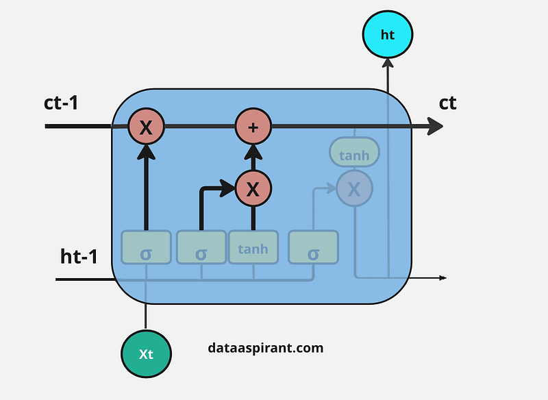
8.2.2 Input Gate

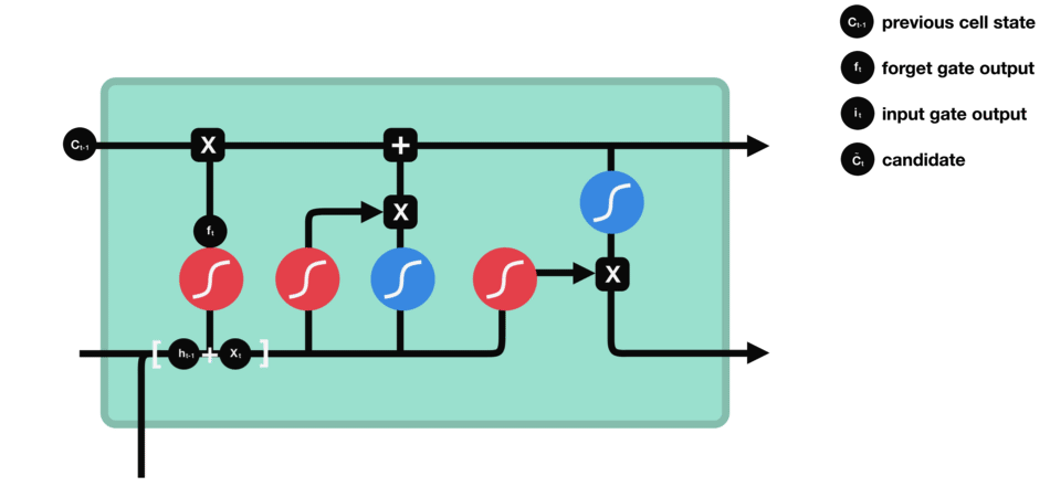
LSTM architecture has an input gate to update the cell state information after the forget gate. Input gates have two kinds of neural net layers one is sigmoid, and another one is tanh. Both network layers take input as previously hidden state information and information from the current input.

Sigmoid network layer results range between 0 and 1, and tanh results range from -1 to 1. The sigmoid layer decides which information is important to keep, and the tanh layer regulates the network.

After applying sigmoid and tanh functions on hidden and current information, then we multiply both outputs. And finally, the sigmoid output will decide which information is important to keep from the tanh output.

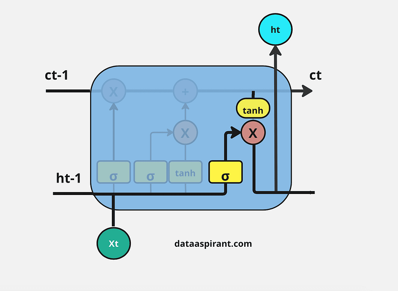
8.2.3 Output Gate

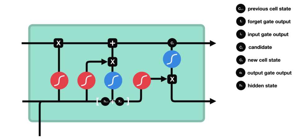
The last gate in the LSTM is the output gate. The output gate’s primary task is to decide what information should be in the next hidden state. This means the output layer’s output is the input to the next hidden state.

The output gate also has two neural net layers, the same as the input gate. But the operations are different. From the input gate, we got updated cell state information.

We have to send hidden state and current input information through the sigmoid layer and updated cell state information through the tanh layer in this output gate. And then multiply both results of the sigmoid and tanh layers.

The final result is sent to the next hidden layer as the input.

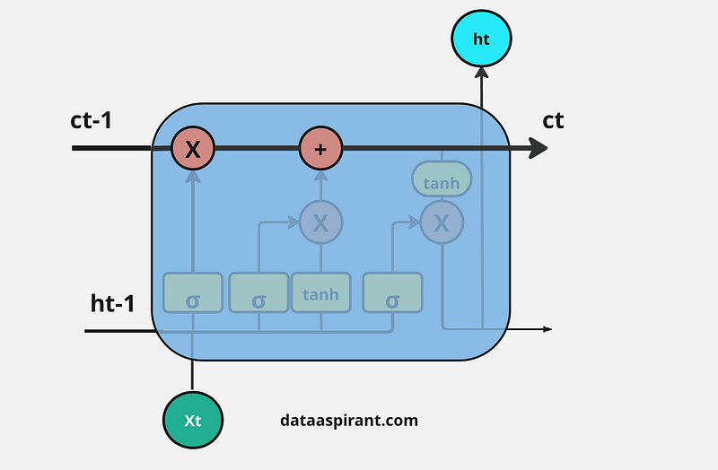
9. Working Procedure of LSTM

The first and foremost step in the LSTM architecture is to decide which information is essential and which is thrown away from the previous cell state. The first gate that does this process in the LSTM is the “Forget gate.”

Forget gate takes input as the previous time step is hidden layer information (ht-1) and present time step input (xt) and sends it through the sigmoid neural net layer.

The result is the vector form, which contains 0 and 1 values. And then, apply a pointwise multiplication operation on the previous cell state (Ct-1) information (vector form) and the output of the sigmoid function (ft).

The final result output of the forget gate 1 represents “completely keep this information,” and 0 represents “don’t keep this information.”

The next step is to decide which information to store in the current cell state (Ct). Another gate will do the task, the second gate in the LSTM architecture is the “Input Gate.”

This whole process of updating the cell state with new important information will be done by using two kinds of activation functions/ neural net layers; their sigmoid neural net and the tanh neural net layer.

First sigmoid net takes the input like the forget gate: previous time step is hidden layer information (ht-1) and current time step (xt).

This process decides which values we’ll update. And then, the tanh neural net also takes the same input as a sigmoid neural net layer. It creates new candidate values in the form of the vector (ct(upper dash)) to regulate the network.

Now we apply pointwise multiplication on the outputs of the sigmoid and tanh layers. After that, we have to perform a pointwise addition operation on the output of the forget gate and the result of the pointwise multiplication in the input gate to update the current cell state information (ct).

The final step in the LSTM architecture is to decide which information we’ll be going to as the output; the final gate that will do this process in the LSTM is the “Output Gate.” This output will be based on our cell state but will be the filtered version.

In this gate, we first apply the sigmoid neural net, which takes input like the previous gates’ sigmoid layer: previous time step hidden layer information(ht-1) and current time input (xt) to decide what parts of the cell state information going to the output.

And then send updated cell state information through the tanh neural net layer to regulate the network (push the values between -1 and 1) and then apply pointwise multiplication on both results of the sigmoid and tanh neural network layers.

This whole process is repeated in every module of the LSTM architecture.

10. Types of LSTM Architectures

LSTM is the most interesting starting point to solve or address sequence prediction problems. Based on the way LSTM networks are used as layers, we can divide LSTM architectures into various kinds of LSTMs.

This section will discuss mostly used five different types of LSTM architectures. These are:

Vanilla LSTM

Vanilla LSTM architecture is the basic LSTM architecture; it has only one single hidden layer and one output layer to predict the results.

Stacked LSTM

Stacked LSTM architecture is the LSTM network model that compresses a list or multiple LSTM layers. Stacked LSTM is also known as the Deep LSTM network model.

In this architecture, every LSTM layer predicts the sequence of outputs to send to the next LSTM layer instead of predicting a single output value. Then the final LSTM layer predicts the single output.

CNN LSTM

CNN LSTM architecture is a combination of CNN and LSTM architectures. This architecture uses the CNN network layer to extract the essential features from the input and then send them to the LSTM layer to support sequence prediction.

An example application for this architecture is generating textual descriptions for the input image or sequences of images like video.

Encoder-Decoder LSTM

Encoder-decoder LSTM architecture is a special kind of LSTM architecture. It is mainly designed to solve sequence-to-sequence problems such as machine translation, speech recognition, etc. Another name for encoder-decoder LSTM is seq2seq (sequence to sequence).

Sequence-to-sequence problems are challenging problems in the Natural language processing field because, in these problems, the number of input and output items can vary.

Encoder-decoder LSTM architecture has an encoder to convert the input to an intermediate encoder vector. Then one decoder transforms the intermediate encoder vector into the final result. Both the encoder and decoder are stacked LSTMs.

Bidirectional LSTM

Bidirectional LSTM architecture is the extension of traditional LSTM architecture. This architecture is more suitable for sequence classification problems such as sentiment classification, intent classification, etc.

Bidirectional LSTM architecture uses two LSTMs instead of one LSTM one is for forwarding direction (from left to right) and another LSTM for backward direction (from right to left).

This architecture can provide more context information to the network than the traditional LSTM because it will gather information of a word from both sides, the left and right sides. It will accelerate the performance of the sequence classification problems.

11. Building an LSTM from Scratch in Python

In this section, we’ll break down the implementation of an LSTM in Python, step by step, referring back to the mathematical foundations and concepts covered earlier in the article. We will train our made-from-scratch model on the Google stock data. The dataset was retrieved from Kaggle, which is free to use for commercial use.

11.1 Imports and Initial Setup

numpy (np) and pandas (pd): Used for all array and data frame operations, which are fundamental in any kind of numerical computation and particularly in the implementation of neural networks.

The classes WeightInitializer, PlotManager, and EarlyStopping are custom classes.

WeightInitializer

import numpy as np
import pandas as pd

from src.model import WeightInitializer
from src.trainer import PlotManager, EarlyStopping

class WeightInitializer:
    def __init__(self, method='random'):
        self.method = method

    def initialize(self, shape):
        if self.method == 'random':
            return np.random.randn(*shape)
        elif self.method == 'xavier':
            return np.random.randn(*shape) / np.sqrt(shape[0])
        elif self.method == 'he':
            return np.random.randn(*shape) * np.sqrt(2 / shape[0])
        elif self.method == 'uniform':
            return np.random.uniform(-1, 1, shape)
        else:
            raise ValueError(f'Unknown initialization method: {self.method}')

WeightInitializer is a custom class that handles the initialization of weights. This is crucial as different initialization methods can significantly affect the convergence behavior of an LSTM.

PlotManager

class PlotManager:
    def __init__(self):
        self.fig, self.ax = plt.subplots(3, 1, figsize=(6, 4))

    def plot_losses(self, train_losses, val_losses):
        self.ax.plot(train_losses, label='Training Loss')
        self.ax.plot(val_losses, label='Validation Loss')
        self.ax.set_title('Training and Validation Losses')
        self.ax.set_xlabel('Epoch')
        self.ax.set_ylabel('Loss')
        self.ax.legend()

    def show_plots(self):
        plt.tight_layout()

Utility class from src.trainer for managing plots, which will enable us to plot train and validation loss.

EarlyStopping

class EarlyStopping:
    """
    Early stopping to stop the training when the loss does not improve after

    Args:
    -----
        patience (int): Number of epochs to wait before stopping the training.
        verbose (bool): If True, prints a message for each epoch where the loss
                        does not improve.
        delta (float): Minimum change in the monitored quantity to qualify as an improvement.
    """
    def __init__(self, patience=7, verbose=False, delta=0):
        self.patience = patience
        self.verbose = verbose
        self.counter = 0
        self.best_score = None
        self.early_stop = False
        self.delta = delta

    def __call__(self, val_loss):
        """
        Determines if the model should stop training.
        
        Args:
            val_loss (float): The loss of the model on the validation set.
        """
        score = -val_loss

        if self.best_score is None:
            self.best_score = score

        elif score < self.best_score + self.delta:
            self.counter += 1
            
            if self.counter >= self.patience:
                self.early_stop = True
        else:
            self.best_score = score
            self.counter = 0    Args:
    -----
        patience (int): Number of epochs to wait before stopping the training.
        verbose (bool): If True, prints a message for each epoch where the loss
                        does not improve.
        delta (float): Minimum change in the monitored quantity to qualify as an improvement.
    """
    def __init__(self, patience=7, verbose=False, delta=0):
        self.patience = patience
        self.verbose = verbose
        self.counter = 0
        self.best_score = None
        self.early_stop = False
        self.delta = delta

Utility class from src.trainer for handling early stopping during training to prevent overfitting. You can learn more about EarlyStopping, and how it’s functionality is extremely useful for deep neural networks in this article:

11.2 LSTM Class

Let’s first take a look at what the whole class looks like, and then break it down into more manageable steps:

class LSTM:
    """
    Long Short-Term Memory (LSTM) network.
    
    Parameters:
    - input_size: int, dimensionality of input space
    - hidden_size: int, number of LSTM units
    - output_size: int, dimensionality of output space
    - init_method: str, weight initialization method (default: 'xavier')
    """
    def __init__(self, input_size, hidden_size, output_size, init_method='xavier'):
        self.input_size = input_size
        self.hidden_size = hidden_size
        self.output_size = output_size
        self.weight_initializer = WeightInitializer(method=init_method)

        # Initialize weights
        self.wf = self.weight_initializer.initialize((hidden_size, hidden_size + input_size))
        self.wi = self.weight_initializer.initialize((hidden_size, hidden_size + input_size))
        self.wo = self.weight_initializer.initialize((hidden_size, hidden_size + input_size))
        self.wc = self.weight_initializer.initialize((hidden_size, hidden_size + input_size))

        # Initialize biases
        self.bf = np.zeros((hidden_size, 1))
        self.bi = np.zeros((hidden_size, 1))
        self.bo = np.zeros((hidden_size, 1))
        self.bc = np.zeros((hidden_size, 1))

        # Initialize output layer weights and biases
        self.why = self.weight_initializer.initialize((output_size, hidden_size))
        self.by = np.zeros((output_size, 1))

    @staticmethod
    def sigmoid(z):
        """
        Sigmoid activation function.
        
        Parameters:
        - z: np.ndarray, input to the activation function
        
        Returns:
        - np.ndarray, output of the activation function
        """
        return 1 / (1 + np.exp(-z))

    @staticmethod
    def dsigmoid(y):
        """
        Derivative of the sigmoid activation function.

        Parameters:
        - y: np.ndarray, output of the sigmoid activation function

        Returns:
        - np.ndarray, derivative of the sigmoid function
        """
        return y * (1 - y)

    @staticmethod
    def dtanh(y):
        """
        Derivative of the hyperbolic tangent activation function.

        Parameters:
        - y: np.ndarray, output of the hyperbolic tangent activation function

        Returns:
        - np.ndarray, derivative of the hyperbolic tangent function
        """
        return 1 - y * y

    def forward(self, x):
        """
        Forward pass through the LSTM network.

        Parameters:
        - x: np.ndarray, input to the network

        Returns:
        - np.ndarray, output of the network
        - list, caches containing intermediate values for backpropagation
        """
        caches = []
        h_prev = np.zeros((self.hidden_size, 1))
        c_prev = np.zeros((self.hidden_size, 1))
        h = h_prev
        c = c_prev

        for t in range(x.shape[0]):
            x_t = x[t].reshape(-1, 1)
            combined = np.vstack((h_prev, x_t))
            
            f = self.sigmoid(np.dot(self.wf, combined) + self.bf)
            i = self.sigmoid(np.dot(self.wi, combined) + self.bi)
            o = self.sigmoid(np.dot(self.wo, combined) + self.bo)
            c_ = np.tanh(np.dot(self.wc, combined) + self.bc)
            
            c = f * c_prev + i * c_
            h = o * np.tanh(c)

            cache = (h_prev, c_prev, f, i, o, c_, x_t, combined, c, h)
            caches.append(cache)

            h_prev, c_prev = h, c

        y = np.dot(self.why, h) + self.by
        return y, caches

    def backward(self, dy, caches, clip_value=1.0):
        """
        Backward pass through the LSTM network.

        Parameters:
        - dy: np.ndarray, gradient of the loss with respect to the output
        - caches: list, caches from the forward pass
        - clip_value: float, value to clip gradients to (default: 1.0)

        Returns:
        - tuple, gradients of the loss with respect to the parameters
        """
        dWf, dWi, dWo, dWc = [np.zeros_like(w) for w in (self.wf, self.wi, self.wo, self.wc)]
        dbf, dbi, dbo, dbc = [np.zeros_like(b) for b in (self.bf, self.bi, self.bo, self.bc)]
        dWhy = np.zeros_like(self.why)
        dby = np.zeros_like(self.by)

        # Ensure dy is reshaped to match output size
        dy = dy.reshape(self.output_size, -1)
        dh_next = np.zeros((self.hidden_size, 1))  # shape must match hidden_size
        dc_next = np.zeros_like(dh_next)

        for cache in reversed(caches):
            h_prev, c_prev, f, i, o, c_, x_t, combined, c, h = cache

            # Add gradient from next step to current output gradient
            dh = np.dot(self.why.T, dy) + dh_next
            dc = dc_next + (dh * o * self.dtanh(np.tanh(c)))

            df = dc * c_prev * self.dsigmoid(f)
            di = dc * c_ * self.dsigmoid(i)
            do = dh * self.dtanh(np.tanh(c))
            dc_ = dc * i * self.dtanh(c_)

            dcombined_f = np.dot(self.wf.T, df)
            dcombined_i = np.dot(self.wi.T, di)
            dcombined_o = np.dot(self.wo.T, do)
            dcombined_c = np.dot(self.wc.T, dc_)

            dcombined = dcombined_f + dcombined_i + dcombined_o + dcombined_c
            dh_next = dcombined[:self.hidden_size]
            dc_next = f * dc

            dWf += np.dot(df, combined.T)
            dWi += np.dot(di, combined.T)
            dWo += np.dot(do, combined.T)
            dWc += np.dot(dc_, combined.T)

            dbf += df.sum(axis=1, keepdims=True)
            dbi += di.sum(axis=1, keepdims=True)
            dbo += do.sum(axis=1, keepdims=True)
            dbc += dc_.sum(axis=1, keepdims=True)

        dWhy += np.dot(dy, h.T)
        dby += dy

        gradients = (dWf, dWi, dWo, dWc, dbf, dbi, dbo, dbc, dWhy, dby)

        # Gradient clipping
        for i in range(len(gradients)):
            np.clip(gradients[i], -clip_value, clip_value, out=gradients[i])

        return gradients

    def update_params(self, grads, learning_rate):
        """
        Update the parameters of the network using the gradients.

        Parameters:
        - grads: tuple, gradients of the loss with respect to the parameters
        - learning_rate: float, learning rate
        """
        dWf, dWi, dWo, dWc, dbf, dbi, dbo, dbc, dWhy, dby = grads

        self.wf -= learning_rate * dWf
        self.wi -= learning_rate * dWi
        self.wo -= learning_rate * dWo
        self.wc -= learning_rate * dWc

        self.bf -= learning_rate * dbf
        self.bi -= learning_rate * dbi
        self.bo -= learning_rate * dbo
        self.bc -= learning_rate * dbc

        self.why -= learning_rate * dWhy
        self.by -= learning_rate * dby

Initialization The __init__ method initializes an LSTM instance with specified sizes for input, hidden, and output layers, and selects a method for weight initialization.

The weights are initialized for the gates (forget wf, input wi, output wo, and cell wc) and for connecting the last hidden state to the output (why). Xavier initialization is often chosen as it's a good default for maintaining the variance of activations across layers.

Biases for all gates and the output layer are initialized to zero. This is a common practice, although sometimes small constants are added to avoid dead neurons at the start.

Forward Pass Method

We start by setting the previous hidden state h_prev and cell state c_prev to zero, which is typical for the first timestep.

def forward(self, x): The input x is processed timestep by timestep, where each timestep updates the gates' activations, the cell state, and the hidden state.

for t in range(x.shape[0]):
    x_t = x[t].reshape(-1, 1)
    combined = np.vstack((h_prev, x_t))

At each time step, the input and the previous hidden state are stacked vertically to form a single combined input for matrix operations. This is crucial for performing the linear transformations efficiently in one go.

f = self.sigmoid(np.dot(self.wf, combined) + self.bf)
    i = self.sigmoid(np.dot(self.wi, combined) + self.bi)
    o = self.sigmoid(np.dot(self.wo, combined) + self.bo)
    c_ = np.tanh(np.dot(self.wc, combined) + self.bc)
    
    c = f * c_prev + i * c_
    h = o * np.tanh(c)

Each gate (forget, input, output) computes its activation using a sigmoid function, influencing how the cell state and the hidden state are updated.

Here, the forget gate (f) determines the amount of the previous cell state to retain. The input gate (i) decides how much of the new candidate cell state (c_) to add. Finally, the output gate (o) calculates what portion of the cell state to output as the hidden state.

The cell state is updated as a weighted sum of the previous state and the new candidate state. The hidden state is derived by passing the updated cell state through a tanh function and then gating it with the output gate.

cache = (h_prev, c_prev, f, i, o, c_, x_t, combined, c, h)
caches.append(cache)

We store relevant values needed for backpropagation in cache. This includes states, gate activations, and inputs.

y = np.dot(self.why, h) + self.by

Finally, the output y is computed as a linear transformation of the last hidden state. The method returns both the output and the cached values for use during backpropagation.

Backward Pass Method

This method is used to calculate gradients of the loss function with respect to the weights and biases of the LSTM. These gradients are necessary for updating the model’s parameters during training.

def backward(self, dy, caches, clip_value=1.0):
    dWf, dWi, dWo, dWc = [np.zeros_like(w) for w in (self.wf, self.wi, self.wo, self.wc)]
    dbf, dbi, dbo, dbc = [np.zeros_like(b) for b in (self.bf, self.bi, self.bo, self.bc)]
    dWhy = np.zeros_like(self.why)
    dby = np.zeros_like(self.by)

All gradients for the weights (dWf, dWi, dWo, dWc, dWhy) and biases (dbf, dbi, dbo, dbc, dby) are initialized to zero. This is necessary because the gradients are accumulated over each timestep in the sequence.

dy = dy.reshape(self.output_size, -1)
dh_next = np.zeros((self.hidden_size, 1))
dc_next = np.zeros_like(dh_next)

Here, we ensure that dy is in the correct shape for matrix operations. dh_next and dc_next store gradients are flowing back from later timesteps.

for cache in reversed(caches):
        h_prev, c_prev, f, i, o, c_, x_t, combined, c, h = cache

The LSTM state and gate activations for each timestep are retrieved from cache. Processing starts from the last timestep and moves backward (reversed(caches)), which is essential for correctly applying the chain rule in recurrent neural networks (Backpropagation Through Time - BPTT).

        dh = np.dot(self.why.T, dy) + dh_next
        dc = dc_next + (dh * o * self.dtanh(np.tanh(c)))
        df = dc * c_prev * self.dsigmoid(f)
        di = dc * c_ * self.dsigmoid(i)
        do = dh * self.dtanh(np.tanh(c))
        dc_ = dc * i * self.dtanh(c_)

dh and dc are gradients of the loss with respect to the hidden state and cell state. Gradients for each gate (df, di, do) and the candidate cell state (dc_) are calculated using the chain rule, involving derivatives of the sigmoid (dsigmoid) and tanh (dtanh) functions, which were discussed in the gating mechanisms.

        dWf += np.dot(df, combined.T)
        dWi += np.dot(di, combined.T)
        dWo += np.dot(do, combined.T)
        dWc += np.dot(dc_, combined.T)
        dbf += df.sum(axis=1, keepdims=True)
        dbi += di.sum(axis=1, keepdims=True)
        dbo += do.sum(axis=1, keepdims=True)
        dbc += dc_.sum(axis=1, keepdims=True)

These lines accumulate the gradients over all timesteps for each weight and bias.

for i in range(len(gradients)):
    np.clip(gradients[i], -clip_value, clip_value, out=gradients[i])

To prevent exploding gradients, we clip the gradients to a specified range (clip_value), which is a common practice in training RNNs.

Parameter Update Method

def update_params(self, grads, learning_rate):
    dWf, dWi, dWo, dWc, dbf, dbi, dbo, dbc, dWhy, dby = grads
    ...
    self.wf -= learning_rate * dWf
    ...

Each weight and bias is updated by subtracting a fraction (learning_rate) of the corresponding gradient. This step adjusts the model parameters to minimize the loss function.

11.3 Training and Validation

class LSTMTrainer:
    """
    Trainer for the LSTM network.

    Parameters:
    - model: LSTM, the LSTM network to train
    - learning_rate: float, learning rate for the optimizer
    - patience: int, number of epochs to wait before early stopping
    - verbose: bool, whether to print training information
    - delta: float, minimum change in validation loss to qualify as an improvement
    """
    def __init__(self, model, learning_rate=0.01, patience=7, verbose=True, delta=0):
        self.model = model
        self.learning_rate = learning_rate
        self.train_losses = []
        self.val_losses = []
        self.early_stopping = EarlyStopping(patience, verbose, delta)

    def train(self, X_train, y_train, X_val=None, y_val=None, epochs=10, batch_size=1, clip_value=1.0):
        """
        Train the LSTM network.

        Parameters:
        - X_train: np.ndarray, training data
        - y_train: np.ndarray, training labels
        - X_val: np.ndarray, validation data
        - y_val: np.ndarray, validation labels
        - epochs: int, number of training epochs
        - batch_size: int, size of mini-batches
        - clip_value: float, value to clip gradients to
        """
        for epoch in range(epochs):
            epoch_losses = []
            for i in range(0, len(X_train), batch_size):
                batch_X = X_train[i:i + batch_size]
                batch_y = y_train[i:i + batch_size]
                losses = []
                
                for x, y_true in zip(batch_X, batch_y):
                    y_pred, caches = self.model.forward(x)
                    loss = self.compute_loss(y_pred, y_true.reshape(-1, 1))
                    losses.append(loss)
                    
                    # Backpropagation to get gradients
                    dy = y_pred - y_true.reshape(-1, 1)
                    grads = self.model.backward(dy, caches, clip_value=clip_value)
                    self.model.update_params(grads, self.learning_rate)

                batch_loss = np.mean(losses)
                epoch_losses.append(batch_loss)

            avg_epoch_loss = np.mean(epoch_losses)
            self.train_losses.append(avg_epoch_loss)

            if X_val is not None and y_val is not None:
                val_loss = self.validate(X_val, y_val)
                self.val_losses.append(val_loss)
                print(f'Epoch {epoch + 1}/{epochs} - Loss: {avg_epoch_loss:.5f}, Val Loss: {val_loss:.5f}')
                
                # Check early stopping condition
                self.early_stopping(val_loss)
                if self.early_stopping.early_stop:
                    print("Early stopping")
                    break
            else:
                print(f'Epoch {epoch + 1}/{epochs} - Loss: {avg_epoch_loss:.5f}')


    def compute_loss(self, y_pred, y_true):
        """
        Compute mean squared error loss.
        """
        return np.mean((y_pred - y_true) ** 2)

    def validate(self, X_val, y_val):
        """
        Validate the model on a separate set of data.
        """
        val_losses = []
        for x, y_true in zip(X_val, y_val):
            y_pred, _ = self.model.forward(x)
            loss = self.compute_loss(y_pred, y_true.reshape(-1, 1))
            val_losses.append(loss)
        return np.mean(val_losses)

The trainer orchestrates the training process over multiple epochs, handling batches of data, and optionally validating the model.

for epoch in range(epochs):
      ...
      for i in range(0, len(X_train), batch_size):
          ...
          for x, y_true in zip(batch_X, batch_y):
              y_pred, caches = self.model.forward(x)
              ...

Each batch of data is fed through the model. The forward pass generates predictions and caches intermediate values for backpropagation.

dy = y_pred - y_true.reshape(-1, 1)
grads = self.model.backward(dy, caches, clip_value=clip_value)
self.model.update_params(grads, self.learning_rate)

After calculating the loss, the gradient with respect to the prediction error (dy) is used to perform backpropagation. The resulting gradients are used to update the model parameters.

print(f'Epoch {epoch + 1}/{epochs} - Loss: {avg_epoch_loss:.5f}')

Training progress is logged to help monitor the model’s performance over time.

11.4 Data Preprocessing

class TimeSeriesDataset:
    """
    Dataset class for time series data.

    Parameters:
    - ticker: str, stock ticker symbol
    - start_date: str, start date for data retrieval
    - end_date: str, end date for data retrieval
    - look_back: int, number of previous time steps to include in each sample
    - train_size: float, proportion of data to use for training
    """
    def __init__(self, start_date, end_date, look_back=1, train_size=0.67):
        self.start_date = start_date
        self.end_date = end_date
        self.look_back = look_back
        self.train_size = train_size

    def load_data(self):
        """
        Load stock data.
        
        Returns:
        - np.ndarray, training data
        - np.ndarray, testing data
        """
        df = pd.read_csv('data/google.csv')
        df = df[(df['Date'] >= self.start_date) & (df['Date'] <= self.end_date)]
        df = df.sort_index()
        df = df.loc[self.start_date:self.end_date]
        df = df[['Close']].astype(float)  # Use closing price
        df = self.MinMaxScaler(df.values)  # Convert DataFrame to numpy array
        train_size = int(len(df) * self.train_size)
        train, test = df[0:train_size,:], df[train_size:len(df),:]
        return train, test
    
    def MinMaxScaler(self, data):
        """
        Min-max scaling of the data.
        
        Parameters:
        - data: np.ndarray, input data
        """
        numerator = data - np.min(data, 0)
        denominator = np.max(data, 0) - np.min(data, 0)
        return numerator / (denominator + 1e-7)

    def create_dataset(self, dataset):
        """
        Create the dataset for time series prediction.

        Parameters:
        - dataset: np.ndarray, input data

        Returns:
        - np.ndarray, input data
        - np.ndarray, output data
        """
        dataX, dataY = [], []
        for i in range(len(dataset)-self.look_back):
            a = dataset[i:(i + self.look_back), 0]
            dataX.append(a)
            dataY.append(dataset[i + self.look_back, 0])
        return np.array(dataX), np.array(dataY)

    def get_train_test(self):
        """
        Get the training and testing data.

        Returns:
        - np.ndarray, training input
        - np.ndarray, training output
        - np.ndarray, testing input
        - np.ndarray, testing output
        """
        train, test = self.load_data()
        trainX, trainY = self.create_dataset(train)
        testX, testY = self.create_dataset(test)
        return trainX, trainY, testX, testY

This class handles fetching and preprocessing data into a format suitable for training the LSTM, including scaling and splitting into training and test sets.

11.5 Model Training

Now let’s leverage all the code defined above to load the dataset, preprocess it, and train our LSTM model.

First, let’s load the dataset:

# Instantiate the dataset
dataset = TimeSeriesDataset( '2010-1-1', '2020-12-31', look_back=1)
trainX, trainY, testX, testY = dataset.get_train_test()

In this instance, it’s configured to fetch historical data for Google (GOOGL) from Kaggle, spanning from January 1, 2010, to December 31, 2020.

look_back=1: This parameter sets the number of past time steps to include in each input sample. Here, each input sample will contain data from 1 previous time step, which means that the model will use data from one day to predict the next.

get_train_test(): This method processes the fetched data, normalizes it, and splits it into training and testing datasets. This is essential for training the model on one segment of the data and validating its performance on another to check for overfitting.

# Reshape input to be [samples, time steps, features]
trainX = np.reshape(trainX, (trainX.shape[0], trainX.shape[1], 1))
testX = np.reshape(testX, (testX.shape[0], testX.shape[1], 1))

This reshaping step adjusts the data format to what the LSTM expects. LSTMs require input to be in the shape of [samples, time steps, features]. Here:

• samples: the number of data points.
• time steps: the number of time steps per sample (look_back).
• features: the number of features per time step (in this case, 1, because we are probably looking at one dimension of data like closing price).

look_back = 1  # Number of previous time steps to include in each sample
hidden_size = 256  # Number of LSTM units
output_size = 1  # Dimensionality of the output space

lstm = LSTM(input_size=1, hidden_size=hidden_size, output_size=output_size)

In this code:

• hidden_size : The number of LSTM units in the hidden layer, which is set to 256. This defines the capacity of the model, with more units potentially capturing more complex patterns but also requiring more computational power and data to train effectively.
• output_size : The output dimensionality, which is 1 in this case, suggests the model predicts a single value per input sample, such as the next day’s stock price.

trainer = LSTMTrainer(lstm, learning_rate=1e-3, patience=50, verbose=True, delta=0.001)
trainer.train(trainX, trainY, testX, testY, epochs=1000, batch_size=32)

Here we set the rate to 1e-3 (0.001). A learning rate that’s too high can cause the model to converge too quickly to a suboptimal solution, and too low a rate can make the training process slow and possibly stuck. We also specified patience to 50, which will stop the model training if the validation loss doesn’t improve for 50 epochs.

The train() method executes the training process over a specified number of epochs and batch sizes. During training, the model will print the model performance every 10 epochs, resulting in an output similar to this one:

Epoch 1/1000 - Loss: 0.25707, Val Loss: 0.43853
Epoch 11/1000 - Loss: 0.06463, Val Loss: 0.06056
Epoch 21/1000 - Loss: 0.05313, Val Loss: 0.02100
Epoch 31/1000 - Loss: 0.04862, Val Loss: 0.01134
Epoch 41/1000 - Loss: 0.04512, Val Loss: 0.00678
Epoch 51/1000 - Loss: 0.04234, Val Loss: 0.00395
Epoch 61/1000 - Loss: 0.04014, Val Loss: 0.00210
Epoch 71/1000 - Loss: 0.03840, Val Loss: 0.00095
Epoch 81/1000 - Loss: 0.03703, Val Loss: 0.00031
Epoch 91/1000 - Loss: 0.03595, Val Loss: 0.00004
Epoch 101/1000 - Loss: 0.03509, Val Loss: 0.00003
Epoch 111/1000 - Loss: 0.03442, Val Loss: 0.00021
Epoch 121/1000 - Loss: 0.03388, Val Loss: 0.00051
Epoch 131/1000 - Loss: 0.03346, Val Loss: 0.00090
Epoch 141/1000 - Loss: 0.03312, Val Loss: 0.00133
Early stopping

Lastly, let’s plot train and validation loss to get a better sense of a possible convergence/divergence. We can achieve that using the following lines of code:

plot_manager = PlotManager()

# Inside your training loop
plot_manager.plot_losses(trainer.train_losses, trainer.val_losses)

# After your training loop
plot_manager.show_plots()

Which will plot a similar chart to the following:

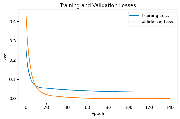
From the graph, we can see that both train and validation drop quickly in the earlier epochs, which suggests our initialization technique (Xavier) may not be ideal for this purpose. Although early stopping is triggered after ~90 epochs achieving some impressive performances, we could try to decrease the learning rate and run it for more epochs. Moreover, we could try to use other techniques like learning rate schedulers or Adam optimization.

12. Gated Recurrent Units (GRUs)

Gated recurrent unit (GRU) was introduced by Cho, et al. in 2014 to solve the vanishing gradient problem faced by standard recurrent neural networks (RNN). GRU shares many properties of long short-term memory (LSTM). Both algorithms use a gating mechanism to control the memorization process.

Imagine you’re trying to learn a song by listening to it repeatedly. A basic RNN might forget the beginning of the song by the time it gets to the end. GRUs solve this problem by using gates that control what information is remembered and what is forgotten.

GRUs simplify the structure of Long Short-Term Memory (LSTM) networks by merging the input and forget gates into a single update gate and adding a reset gate. This makes them faster to train and easier to work with, while still keeping the ability to remember important information for a long time.

Update Gate: This gate decides how much of the past information should be carried forward to the future.

Reset Gate: This gate determines how much of the past information to forget.

These gates help GRUs maintain a balance between remembering important details and forgetting unimportant ones, similar to how you might focus on remembering the melody of a song while ignoring the background noise.

GRUs are great for tasks where data comes in sequences, like predicting the stock market, understanding language, or even generating music. They can learn patterns in data by keeping track of past information and using it to make better predictions. This makes them incredibly useful for any application where understanding the context from previous data points is crucial.

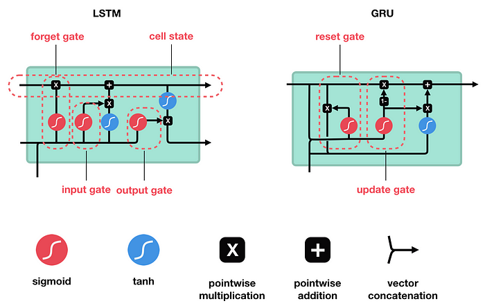
12.1 Comparison with LSTMs and Vanilla RNNs

To understand where GRUs fit in, let’s compare them with LSTMs and Vanilla RNNs.

Vanilla RNNs Think of Vanilla RNNs as the basic version of recurrent neural networks. They work by passing information from one time step to the next, like a relay race where each runner passes the baton to the next. However, they have a big flaw: they tend to forget things over long sequences. This is due to the vanishing gradient problem, which makes it hard for them to learn long-term dependencies in data.

LSTMs Long Short-Term Memory Networks were designed to fix this problem. They use a more complex structure with three types of gates: input, forget, and output gates. These gates act like a sophisticated filing system, deciding what information to keep, what to update, and what to discard. This allows LSTMs to remember important information for long periods, making them great for tasks where context over many time steps is crucial, like understanding paragraphs of text or recognizing patterns in long time series.

GRUs Gated Recurrent Units are a streamlined version of LSTMs. They simplify things by combining the input and forget gates into a single update gate, and they also have a reset gate. This makes GRUs less computationally intensive and faster to train than LSTMs, while still being able to handle long-term dependencies effectively.

12.2 What makes GRU special and more effective than traditional RNN?

GRU supports gating and a hidden state to control the flow of information. To solve the problem that comes up in RNN, GRU uses two gates: the update gate and the reset gate.

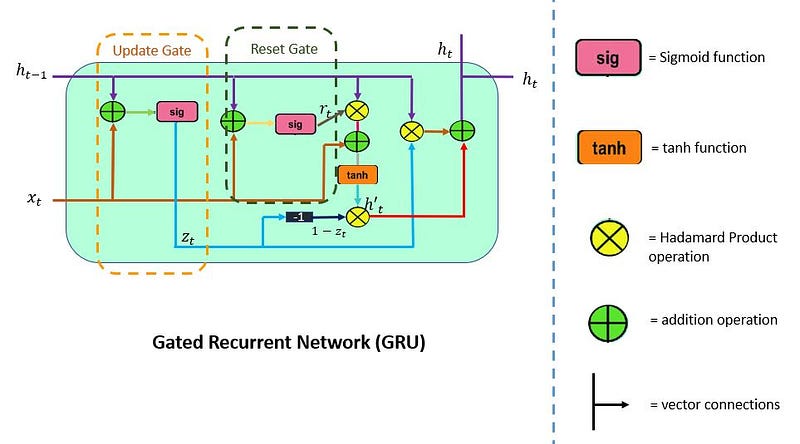
You can consider them as two vector entries (0,1) that can perform a convex combination. These combinations decide which hidden state information should be updated (passed) or reset the hidden state whenever needed. Likewise, the network learns to skip irrelevant temporary observations.

LSTM consists of three gates: the input gate, the forget gate, and the output gate. Unlike LSTM, GRU does not have an output gate and combines the input and the forget gate into a single update gate.

Let’s learn more about the update and reset gates.

12.2.1 Update Gate

The update gate (z_t) is responsible for determining the amount of previous information (prior time steps) that needs to be passed along the next state. It is an important unit. The below schema shows the arrangement of the update gate.

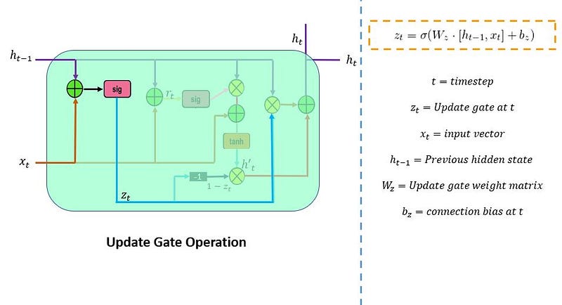
Here, x_t is the input vector served in the network unit. It is multiplied by its parameter weight (W_z) matrices. Thet_1 in h(t_1) signifies that it holds the information of the previous unit and it’s multiplied by its weight. Next, the values from these parameters are added and are passed through the sigmoid activation function. Here, the sigmoid function would generate values between 0 and 1 limit.

12.2.2 Reset Gate

The reset gate (r_t) is used from the model to decide how much of the past information is needed to neglect. The formula is the same as the update gate. There is a difference in their weights and gate usage, which is discussed in the following section. The below schema represents the reset gate.

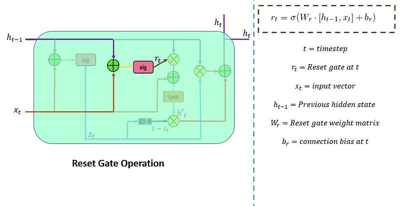
There are two inputs,x_t and h_t-1. Multiply by their weights, apply point-by-point addition, and pass it through sigmoid function.

13. Gates in Action

First, the reset gate stores the relevant information from the past time step into the new memory content. Then it multiplies the input vector and hidden state with their weights. Second, it calculates element-wise multiplication (Hadamard) between the reset gate and previously hidden state multiple. After summing up, the above steps non-linear activation function is applied to results, and it produces h’_t.

Consider a scenario in which a customer reviews a resort: “It was late at night when I reached here.” After a couple of lines, the review ends with, “I enjoyed the stay as the room was comfortable. The staff was friendly.” To determine the customer’s satisfaction level, you will need the last two lines of the reviews. The model will scan the whole review to the end and assign a reset gate vector value close to ‘0’.

That means it will neglect the past lines and focus only on the last sentences.

Refer to the illustration below.

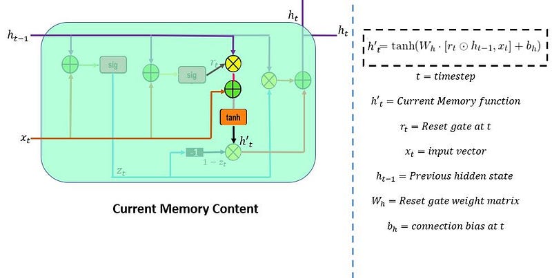
This is the last step. In the final memory at the current time step, the network needs to calculate h_t. Here, the update gate will play a vital role. This vector value will hold information for the current unit and pass it down to the network. It will determine which information to collect from current memory content (h’t) and previous timesteps h(t-1). Element-wise multiplication (Hadamard) is applied to the update gate and h(t-1), and summing it with the Hadamard product operation between (1-z_t) and h’(t).

Revisiting the example of the resort review: This time the relevant information for prediction is mentioned at the beginning of the text. The model would set the update gate vector value close to 1. At the current time step, 1-z_t will be close to 0, and it will ignore the chunk of the last part of the review. Refer to the image below.

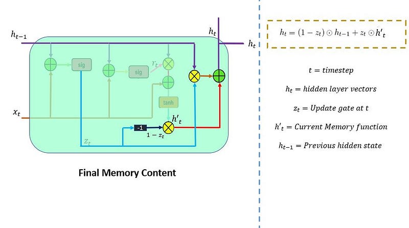
Following through, you can see z_t is used to calculate 1-z_t which, combined with h’t to produce results. Hadamard product operation is carried out between h(t-1) and z_t. The output of the product is given as the input to the point-wise addition with h’t to produce the final results in the hidden state.

14. Implementation of a Simple GRU

To reinforce the concepts we’ve covered, let’s take a hands-on approach and implement a basic Gated Recurrent Unit (GRU) from scratch in Python.

The following code snippet illustrates a simplified GRU class, highlighting the essential functionalities of both forward and backward passes within the GRU architecture.

import numpy as np

class SimpleGRU:
    def __init__(self, input_size, hidden_size, output_size):
        self.input_size = input_size
        self.hidden_size = hidden_size
        self.output_size = output_size

        # Initialize weights and biases
        self.W_z = np.random.randn(hidden_size, input_size)
        self.U_z = np.random.randn(hidden_size, hidden_size)
        self.b_z = np.zeros((hidden_size, 1))
        
        self.W_r = np.random.randn(hidden_size, input_size)
        self.U_r = np.random.randn(hidden_size, hidden_size)
        self.b_r = np.zeros((hidden_size, 1))
        
        self.W_h = np.random.randn(hidden_size, input_size)
        self.U_h = np.random.randn(hidden_size, hidden_size)
        self.b_h = np.zeros((hidden_size, 1))
        
        self.W_y = np.random.randn(output_size, hidden_size)
        self.b_y = np.zeros((output_size, 1))

    def sigmoid(self, x):
        return 1 / (1 + np.exp(-x))
    
    def tanh(self, x):
        return np.tanh(x)
    
    def softmax(self, x):
        exp_x = np.exp(x - np.max(x))
        return exp_x / exp_x.sum(axis=0, keepdims=True)

    def forward(self, x):
        T = len(x)
        h = np.zeros((self.hidden_size, 1))
        y_list = []

        for t in range(T):
            x_t = x[t].reshape(-1, 1)  # Reshape input to column vector

            # Update gate
            z = self.sigmoid(np.dot(self.W_z, x_t) + np.dot(self.U_z, h) + self.b_z)

            # Reset gate
            r = self.sigmoid(np.dot(self.W_r, x_t) + np.dot(self.U_r, h) + self.b_r)

            # Candidate hidden state
            h_tilde = self.tanh(np.dot(self.W_h, x_t) + np.dot(self.U_h, r * h) + self.b_h)

            # Hidden state update
            h = (1 - z) * h + z * h_tilde

            # Output
            y = np.dot(self.W_y, h) + self.b_y
            y_list.append(y)

        return y_list

    def backward(self, x, y_list, target):
        T = len(x)
        dW_z = np.zeros_like(self.W_z)
        dU_z = np.zeros_like(self.U_z)
        db_z = np.zeros_like(self.b_z)
        
        dW_r = np.zeros_like(self.W_r)
        dU_r = np.zeros_like(self.U_r)
        db_r = np.zeros_like(self.b_r)
        
        dW_h = np.zeros_like(self.W_h)
        dU_h = np.zeros_like(self.U_h)
        db_h = np.zeros_like(self.b_h)
        
        dW_y = np.zeros_like(self.W_y)
        db_y = np.zeros_like(self.b_y)
        
        dh_next = np.zeros_like(y_list[0])

        for t in reversed(range(T)):
            dy = y_list[t] - target[t]
            dW_y += np.dot(dy, np.transpose(h))
            db_y += dy
            
            dh = np.dot(np.transpose(self.W_y), dy) + dh_next
            
            dh_tilde = dh * (1 - self.sigmoid(np.dot(self.W_z, x[t].reshape(-1, 1)) + np.dot(self.U_z, h) + self.b_z))
            dW_h += np.dot(dh_tilde, np.transpose(x[t].reshape(1, -1)))
            db_h += dh_tilde
            
            dr = np.dot(np.transpose(self.W_h), dh_tilde)
            dU_h += np.dot(dr * h * (1 - self.tanh(np.dot(self.W_h, x[t].reshape(-1, 1)) + np.dot(self.U_h, r * h) + self.b_h)), np.transpose(h))
            dW_h += np.dot(dr * h * (1 - self.tanh(np.dot(self.W_h, x[t].reshape(-1, 1)) + np.dot(self.U_h, r * h) + self.b_h)), np.transpose(x[t].reshape(1, -1)))
            db_h += dr * h * (1 - self.tanh(np.dot(self.W_h, x[t].reshape(-1, 1)) + np.dot(self.U_h, r * h) + self.b_h))
            
            dz = np.dot(np.transpose(self.U_r), dr * h * (self.tanh(np.dot(self.W_h, x[t].reshape(-1, 1)) + np.dot(self.U_h, r * h) + self.b_h) - h_tilde))
            dU_z += np.dot(dz * h * z * (1 - z), np.transpose(h))
            dW_z += np.dot(dz * h * z * (1 - z), np.transpose(x[t].reshape(1, -1)))
            db_z += dz * h * z * (1 - z)
            
            dh_next = np.dot(np.transpose(self.U_z), dz * h * z * (1 - z))
        
        return dW_z, dU_z, db_z, dW_r, dU_r, db_r, dW_h, dU_h, db_h, dW_y, db_y

    def update_parameters(self, dW_z, dU_z, db_z, dW_r, dU_r, db_r, dW_h, dU_h, db_h, dW_y, db_y, learning_rate):
        self.W_z -= learning_rate * dW_z
        self.U_z -= learning_rate * dU_z
        self.b_z -= learning_rate * db_z
        
        self.W_r -= learning_rate * dW_r
        self.U_r -= learning_rate * dU_r
        self.b_r -= learning_rate * db_r
        
        self.W_h -= learning_rate * dW_h
        self.U_h -= learning_rate * dU_h
        self.b_h -= learning_rate * db_h
        
        self.W_y -= learning_rate * dW_y
        self.b_y -= learning_rate * db_y

# Example usage
input_size = 4
hidden_size = 3
output_size = 2

gru = SimpleGRU(input_size, hidden_size, output_size)

# Generate random data
sequence_length = 5
data = [np.random.randn(input_size) for _ in range(sequence_length)]
target = [np.random.randn(output_size) for _ in range(sequence_length)]

# Forward pass
y_list = gru.forward(data)

# Backward pass
dW_z, dU_z, db_z, dW_r, dU_r, db_r, dW_h, dU_h, db_h, dW_y, db_y = gru.backward(data, y_list, target)

# Update weights and biases
learning_rate = 0.1
gru.update_parameters(dW_z, dU_z, db_z, dW_r, dU_r, db_r, dW_h, dU_h, db_h, dW_y, db_y, learning_rate)

In the implementation above, we’ve introduced a simplified SimpleGRU class to offer insights into the core mechanics of a GRU. The example usage demonstrates how to initialize the GRU, create random data for input sequences and target outputs, perform forward and backward passes, and subsequently update the weights and biases using the computed gradients.

14.1 Pros and Cons of GRUs

Advantages of GRUs

1. Sequential Data Modeling: GRUs excel at handling sequences, making them well-suited for tasks like language processing, speech recognition, and time series analysis.
2. Variable-Length Input: GRUs can work with sequences of varying lengths, accommodating applications where inputs have different sizes.
3. Computationally Efficient: Compared to more complex recurrent architectures like LSTMs, GRUs tend to be computationally more efficient due to their simpler design.
4. Mitigating Vanishing Gradient: GRUs address the vanishing gradient problem more effectively than traditional RNNs, allowing them to capture longer-term dependencies in data.

Limitations of GRUs

1. Limited Long-Term Memory: While GRUs are better at capturing long-term dependencies than standard RNNs, they may not be as effective as LSTMs for very long sequences with complex dependencies.
2. Less Expressive: GRUs might not capture intricate patterns as effectively as LSTMs in some scenarios, particularly when modeling highly complex sequences.
3. Specific Applications: For tasks that require explicit memory control or complex context modeling, LSTMs or more advanced architectures may be more suitable.

14.2 Choosing Between GRUs and LSTMs

The decision between using Gated Recurrent Units (GRUs) or Long Short-Term Memory (LSTM) networks depends on your specific problem and dataset. Here are some considerations:

Use GRUs When:

• Computational Resources are Limited: GRUs are computationally less intensive compared to LSTMs, making them a preferred choice when resource constraints exist.
• Simplicity Matters: If you want a simpler model that still captures sequential dependencies reasonably well, GRUs are a good option.
• Shorter Sequences: For tasks involving sequences with shorter dependencies, GRUs can provide adequate performance without the need for LSTM’s complex memory management.

Use LSTMs When:

• Capturing Long-Term Dependencies: LSTMs are better suited for tasks where capturing long-range dependencies is crucial, such as language modeling, speech recognition, and certain time series predictions.
• Fine-Grained Memory Control: LSTMs offer more explicit control over memory, making them a better choice when precise memory handling is required.
• Complex Sequences: If your data exhibits intricate sequential patterns and dependencies, LSTMs are often more effective at modeling these complexities.

In practice, it’s a good idea to experiment with both GRUs and LSTMs on your specific task to determine which architecture performs better. Sometimes, the choice between the two comes down to empirical testing and validation on your dataset.

15. Conclusion

In this article, we explored Recurrent Neural Networks (RNNs), delving into their core mechanics, training challenges, and advanced designs that enhance their performance. Here’s a quick overview:

We broke down the structure of RNNs, emphasizing their ability to process sequences through internal memory states. Key processes like the forward pass and Backpropagation Through Time (BPTT) were discussed, explaining how RNNs handle sequential data.

We also highlighted major training challenges, including vanishing and exploding gradients, which can disrupt learning. To address these issues, we explored solutions like gradient clipping and initialization strategies, which help stabilize training and improve the network’s ability to learn from longer sequences.

Gated Recurrent Units (GRUs) are a powerful variant of RNNs designed for efficient sequential data processing. They effectively mitigate issues like vanishing gradients and excel at capturing dependencies in sequences, making them ideal for tasks such as natural language processing, speech recognition, and time series analysis.

GRUs use a gating mechanism to control the flow of information, allowing them to capture long-term dependencies while maintaining computational efficiency. Understanding the architecture and mathematics behind GRUs is key to utilizing them effectively in machine learning tasks.

When choosing between GRUs and LSTMs, several factors come into play, including data complexity, computational resources, and the length of dependencies to be modeled. Both architectures have their strengths and weaknesses, so the best choice depends on the specific requirements of your task.

16. Test your Knowledge!

1. Can you explain the role of the loss function and optimizer in the training of a neural network, specifically how they interact during backpropagation and gradient descent? -Expected Answer: The loss function measures the difference between the predicted and actual outputs. During backpropagation, the gradient of the loss concerning each weight is calculated. The optimizer, such as Adam or SGD, updates the weights using these gradients. Gradient descent ensures that the model moves towards the optimal weights, but issues like vanishing or exploding gradients can arise depending on the architecture and depth.

2. Why might a smaller batch size result in noisier gradient updates? What is the trade-off between batch size and computational efficiency? - Expected Answer: A smaller batch size results in noisier gradients because each batch may not represent the entire data distribution well, which can lead to more stochastic updates. However, this noise can also help the model escape local minima. The trade-off is that smaller batch sizes may increase training time due to more frequent updates, but they reduce memory requirements and can generalize better.

3. How does a convolutional neural network (CNN) differ from a recurrent neural network (RNN), and in what types of problems is each architecture most appropriate? - Expected Answer: CNNs are used primarily for spatial data (like images), where the local connectivity and weight-sharing make them efficient for detecting patterns in images. RNNs, on the other hand, are designed for sequential data (like time-series or natural language) where temporal dependencies are important. CNNs are ineffective for maintaining sequence context, which is crucial for RNN tasks like language modeling or sequence prediction.

4. What are the inherent challenges of dealing with sequential data in RNNs, especially for long sequences? - Expected Answer: RNNs struggle with long sequences due to the vanishing gradient problem, where gradients shrink exponentially as they are propagated back through time. This makes it difficult for the network to learn long-term dependencies. Furthermore, the network may become biased toward more recent inputs, ignoring earlier relevant information.

5. Can you explain why RNNs are a better choice than feedforward neural networks for sequential tasks, and how do they process information differently? - Expected Answer: Feedforward networks treat all inputs independently and thus fail to capture temporal dependencies. RNNs, in contrast, maintain a hidden state across time steps, allowing them to learn from prior inputs, which is essential for tasks like language modeling or time-series prediction. This ability to maintain a “memory” of past data gives RNNs an edge in sequential tasks.

6. How does an RNN handle variable-length input sequences, and what impact does padding have on the performance of RNNs? - Expected Answer: RNNs can handle variable-length input sequences by processing one timestep at a time. However, padding is used to standardize input lengths for batching, which introduces additional steps where no meaningful information is present. This can result in inefficiencies, as the model may waste resources processing padded steps. Attention mechanisms or masked loss functions are often used to address this.

7. What is meant by unfolding an RNN in time, and how does it impact the complexity of training and backpropagation? - Expected Answer: Unfolding an RNN in time means representing the network across time steps, where each step corresponds to a recurrent layer. This results in each layer sharing the same weights across time steps. The computational complexity increases significantly with the length of the sequence, making training more challenging due to issues like exploding and vanishing gradients. Backpropagation Through Time (BPTT) is required for calculating gradients, which increases memory and computational demand.

8. What are the main challenges in performing BPTT, and how does it differ from standard backpropagation? - Expected Answer: The key challenge of BPTT is that it must propagate gradients through multiple time steps, which can exacerbate issues like vanishing or exploding gradients. Unlike standard backpropagation, BPTT operates over temporal sequences, which increases memory consumption and computational complexity. To address this, techniques like truncated BPTT are used, where the gradient is only propagated over a limited number of steps.

9. What causes the vanishing and exploding gradient problem in RNNs, and how can it be diagnosed during training? - Expected Answer: The vanishing gradient problem occurs when the gradients become too small, particularly in deep networks, making it hard for the model to learn long-term dependencies. The exploding gradient problem arises when gradients grow exponentially, causing instability in weight updates. This can be diagnosed by monitoring the gradients during training — if they become very small or very large, it’s an indicator of one of these problems.

10. How would you identify that your RNN is suffering from vanishing or exploding gradients, and what steps would you take to resolve it? - Expected Answer: You can identify vanishing or exploding gradients by tracking the magnitude of the gradients during training. If they tend to diminish towards zero or grow uncontrollably, it’s a sign of gradient problems. Solutions include using techniques like gradient clipping (for exploding gradients), employing architectures like LSTMs or GRUs (which help mitigate vanishing gradients), and selecting appropriate activation functions like ReLU or its variants.

11. Why are LSTMs more effective than vanilla RNNs for long-term dependencies, and how do they combat the vanishing gradient problem? - Expected Answer: LSTMs are equipped with a memory cell that can maintain information over long time intervals. The forget, input, and output gates in LSTMs control the flow of information, allowing them to retain relevant information while discarding irrelevant data. These gates help LSTMs combat the vanishing gradient problem by ensuring that the memory cell retains information that is important for long-term dependencies, while still allowing for backpropagation of meaningful gradients.

12. Explain how the forget, input, and output gates work within an LSTM. - Expected Answer: The forget gate decides what information should be discarded from the memory cell. The input gate determines which new information should be added. The output gate controls what information from the current cell state should be used as the hidden state for the next time step. These gates, combined, allow LSTMs to effectively maintain, update, and output information over long sequences.

13. How do GRUs differ from LSTMs, and in which scenarios would you prefer using GRUs over LSTMs? - Expected Answer: GRUs have a simpler architecture compared to LSTMs. They combine the forget and input gates into a single “update gate” and lack an explicit memory cell. This makes GRUs faster and less computationally expensive while performing similarly in many tasks. GRUs are often preferred when training data is limited or when computational efficiency is a priority.

14. What are the key challenges in implementing RNNs or LSTMs from scratch in terms of gradient calculations, training time, and optimization? - Expected Answer: Implementing RNNs or LSTMs requires careful handling of the gradient flow across time steps, which can be computationally expensive due to BPTT. Managing the vanishing or exploding gradient problem is a significant challenge. Optimizing training time requires careful tuning of hyperparameters such as learning rate, batch size, and sequence length. Additionally, ensuring that the architecture can generalize well across various types of sequential data requires effective regularization techniques like dropout.

15. How does gradient clipping help mitigate exploding gradient issues in RNNs, and how would you implement it in practice? - Expected Answer: Gradient clipping limits the magnitude of gradients during backpropagation to prevent them from growing too large and destabilizing training. It can be implemented by setting a threshold value and ensuring that any gradient above this value is clipped. In PyTorch, for instance, you can use `torch.nn.utils.clip_grad_norm_` to clip gradients.

16. Why do non-saturating activation functions like ReLU or Leaky ReLU help with vanishing gradients in deep neural networks, and are they effective in RNNs? - Expected Answer: Non-saturating activation functions like ReLU or Leaky ReLU avoid the saturation problem that occurs with functions like sigmoid or tanh, where gradients become too small. While ReLU is effective in feedforward networks, it can cause dead neurons in RNNs, so Leaky ReLU or variants like ELU are often preferred in RNN architectures to maintain some flow of gradients.

17. What is meant by the memory capacity of an RNN, and how is it related to the number of recurrent layers or time steps unfolded? - Expected Answer: The memory capacity of an RNN refers to its ability to retain information over long sequences. It is influenced by the number of time steps unfolded, the hidden state size, and the recurrence depth. As the network is unfolded over more time steps, it can theoretically retain more information, but vanishing gradients can limit the practical capacity.

18. How does truncated BPTT work, and why might it be used instead of standard BPTT? - Expected Answer: Truncated BPTT limits the number of time steps over which gradients are propagated backward. This reduces the computational cost and mitigates the vanishing gradient problem for long sequences. It’s used when sequences are too long for standard BPTT to be practical or when training efficiency is prioritized.

19. How do the gates in LSTMs specifically address the vanishing gradient problem, allowing for long-term dependency learning? - Expected Answer: LSTMs use gating mechanisms — specifically, the forget, input, and output gates — to control the flow of information. The cell state in LSTMs allows gradients to flow unchanged over long sequences, helping to prevent vanishing gradients. The forget gate ensures that irrelevant information is discarded, while the input gate ensures that useful information is retained.

20. In terms of computational complexity, how do GRUs compare to LSTMs, and what is the trade-off between the two architectures? - Expected Answer: GRUs are simpler than LSTMs as they have fewer gates (two vs. three) and no separate memory cell, leading to fewer parameters and faster training times. However, LSTMs offer more control over the retention of information through their additional gate (forget gate), which can be beneficial for more complex tasks that require fine-grained memory management.

21. Why is it common practice to initialize the forget gate bias to a high value in LSTMs, and how does this affect training? - Expected Answer: Initializing the forget gate bias to a high value (e.g., 1 or higher) encourages the model to retain more information in the initial training stages. This prevents early forgetting of relevant information and helps the model learn long-term dependencies before it starts deciding to forget certain parts of the input.

22. Why might GRUs be preferred over LSTMs in resource-constrained environments, and how does this choice affect the quality of the model’s predictions? - Expected Answer: GRUs are computationally more efficient due to fewer gates and a simpler structure. In resource-constrained environments, this leads to faster training and lower memory consumption. While GRUs are often as effective as LSTMs, they may not capture long-term dependencies as effectively in more complex tasks, potentially affecting the prediction quality.

23. How does a bidirectional RNN differ from a standard RNN, and when would you use it in sequence tasks? - Expected Answer: A bidirectional RNN processes sequences in both forward and reverse directions, allowing it to capture information from both past and future time steps. This is particularly useful in tasks where context from the entire sequence is important, such as in language translation or named entity recognition.

24. How does using dropout in RNNs differ from dropout in feedforward networks, and what precautions should you take when applying dropout to recurrent layers? - Expected Answer: Applying dropout in RNNs can be tricky because standard dropout would apply at every time step, which could disrupt the temporal continuity of the hidden states. Instead, recurrent dropout is used, where dropout is applied only between layers (not between time steps) to maintain temporal coherence while still providing regularization.

25. Why is proper weight initialization important in RNNs, and what are the best practices for initializing weights to avoid exploding or vanishing gradients? - Expected Answer: Proper weight initialization is crucial to ensure stable gradient flow in RNNs. Weights should be initialized using methods like Xavier or He initialization depending on the activation functions used. Poor initialization can exacerbate the vanishing/exploding gradient problem, leading to inefficient training.

26. How does initializing the hidden state affect the performance of RNNs during training, and why might you choose to initialize states to zero or other learned values? - Expected Answer: The hidden state in RNNs is typically initialized to zero, but this can lead to slow convergence if the initial state is far from the optimal trajectory. Alternatively, learned initial states or random initialization can provide better starting points for optimization. Learned initialization often improves convergence, especially in tasks where the initial state carries meaningful information.

DIY

1. What will happen if the activation function is removed from a neural network?
2. When building a neural network, what is the benefit of normalizing inputs?
3. What is the difference between a loss function and a cost function?
4. Is text processing possible with CNN? Why is it not preferred and RNNs more preferred for it?
5. Can we perform image classification with RNNs? Justify your answer.
6. What is the dimension of input that we send into RNNs or LSTMs?
7. Calculate the number of parameters in an RNN that has 5 input nodes, 1 Hidden Layer with 3 hidden Nodes.
8. If we use an RNN to predict the next character in a text sequence, what is the required dimension for any output?
9. Why can RNNs express the conditional probability of a token at some time step based on all the previous tokens in the text sequence?
10. What happens to the gradient if you backpropagate through a long sequence?
11. Besides gradient clipping, can you think of any other methods to cope with gradient explosion in recurrent neural networks?
12. Compare the computational cost for GRUs, LSTMs, and regular RNNs for a given hidden dimension. Pay special attention to the training and inference cost.
13. Since the candidate memory cell ensures that the value range is between −1 and 1 by using the tanh function, why does the hidden state need to use the tanh function again to ensure that the output value range is between −1 and 1?
14. What happens if you implement only parts of a GRU, e.g., with only a reset gate or only an update gate?

Thank you for reading!

If this guide has enhanced your understanding of Python and Machine Learning:

• Please show your support with a clap 👏 or several claps!
• Your claps help me create more valuable content for our vibrant Python or ML community.
• Feel free to share this guide with fellow Python or AI / ML enthusiasts.
• Your feedback is invaluable — it inspires and guides my future posts.

Connect with me!

Vipra