Overview of a Neural Network’s Learning Process

Neural Networks and Deep Learning Course: Part 8

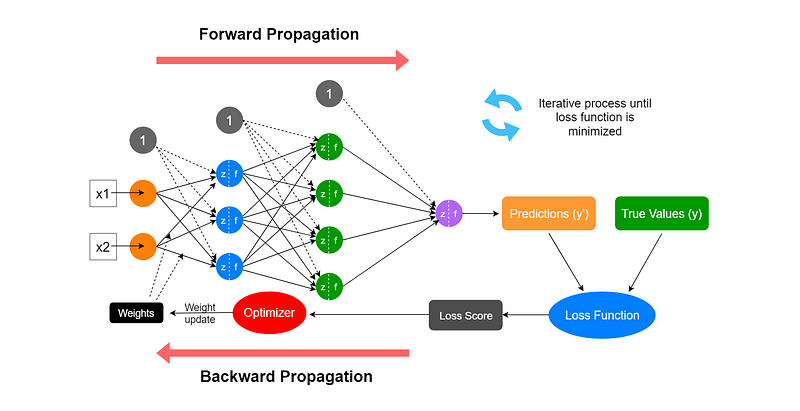
The learning (training) process of a neural network is an iterative process in which the calculations are carried out forward and backward through each layer in the network until the loss function is minimized.

The entire learning process can be divided into three main parts:

• Forward propagation (Forward pass)
• Calculation of the loss function
• Backward propagation (Backward pass/Backpropagation)

We’ll begin with forward propagation.

Forward propagation

A neural network is made of multiple neurons (perceptrons) and these neurons are stacked into layers. The connections between the layers occurred through the parameters (represented by arrows) of the network. The parameters are weights and biases.

The weights control the level of importance of each input while biases determine how easily a neuron fires or activates.

First, we assign non-zero random values to weights and biases. This is called parameter initialization of the network. Based on these assigned values and the input values, we perform the following calculations in each neuron of the network.

• Calculation of neuron's linear unction
• Calculation of neuron’s activation function

These calculations occur throughout the entire network. After completing the calculations in the output layer node(s), we get the final output of the forward propagation part in the first iteration.

In the forward propagation, calculations are made from the input layer to the output layer (left to right) through the network.

Calculation of the loss function

The final output performed in the forward propagation is called the predicted value. This value should be compared with the corresponding ground-truth value (real value) to measure the performance of the neural network. This is where the loss function (also called objective function or cost function) comes into play.

The loss function computes a score called the loss score between the predicted values and ground truth values. This is also known as the error of the model. The loss function captures how well the model performs in each iteration. We use the loss score as a feedback signal to update parameters in the backpropagation part.

The ideal value of the loss function is zero (0). Our goal is to minimize the loss function close to 0 in each iteration so that the model will make better predictions that are close to ground truth values.

Here is a list of commonly used loss functions in neural network training.

• Mean Squared Error (MSE) — This is used to measure the performance of regression problems.
• Mean Absolute Error (MAE) — This is used to measure the performance of regression problems.
• Mean Absolute Percentage Error — This is used to measure the performance of regression problems.
• Huber Loss — This is used to measure the performance of regression problems.
• Binary Cross-entropy (Log Loss) — This is used to measure the performance of binary (two-class) classification problems.
• Multi-class Cross-entropy/Categorical Cross-entropy — This is used to measure the performance of multi-class (more than two classes) classification problems.

A complete list of available loss functions in Keras can be found here.

Backward propagation

In the first iteration, the predicted values are far from the ground truth values and the distance score will be high. This is because we initially assigned arbitrary values to the network’s parameters (weights and biases). Those values are not optimal values. So, we need to update the values of these parameters in order to minimize the loss function. The process of updating network parameters is called parameter learning or optimization which is done using an optimization algorithm (optimizer) that implements backpropagation.

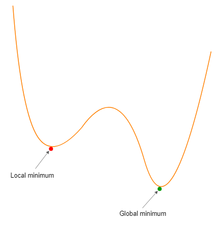
The objective of the optimization algorithm is to find the global minima where the loss function has its minimum value. However, it is a real challenge for an optimization algorithm to find the global minimum of a complex loss function by avoiding all the local minima. If the algorithm is stopped at a local minimum, we’ll not get the minimum value for the loss function. Therefore, our model will not perform well.

Here is a list of commonly used optimizers in neural network training.

• Gradient Descent
• Stocasticc Gradeint Descent (SGD)
• Adam
• Adagrad
• Adadelta
• Adamax
• Nadam
• Ftrl
• Root Mean Squared Propagation (RMSProp)

In the backward propagation, the partial derivatives (gradients) of the loss function with respect to the model parameters in each layer are calculated. This is done by applying the chain rule of calculus.

The derivative of the loss function is its slope which provides us with the direction that we should need to consider for updating (changing) the values of the model parameters.

The neural network libraries in Keras provide automatic differentiation. This means, after you define the neural network architecture, the libraries automatically calculate all of the derivates needed for backpropagation.

In the backward propagation, calculations are made from the output layer to the input layer (right to left) through the network.

The batch size and epochs

We do not usually use all training samples (instances/rows) in one iteration during the neural network training. Instead, we specify the batch size which determines the number of training samples to be propagated (forward and backward) during training.

An epoch is an iteration over the entire training dataset.

For example, let’s say we have a dataset of 1000 training samples and we choose a batch size of 10 and epochs of 20. In this case, our dataset will be divided into 100 (1000/10) batches each with 10 training samples. According to this setting, the algorithm takes the first 10 training samples from the dataset and trains the model. Next, it takes the second 10 training samples and trains the model and so on. Since there is a total of 100 batches, the model parameters will be updated 100 times in each epoch of optimization. This means that one epoch involves 100 batches or 100 times parameter updates. Since the number of epochs is 20, the optimizer passes through the entire training dataset 20 times giving a total of 2000 (100x20) iterations!

This is the end of today’s post. Thanks for reading!

Never miss a great story again by subscribing to my email list. You’ll receive every story in your inbox as soon as I hit the publish button.

If you’d like, you can sign up for a membership to get full access to every story I write and I will receive a portion of your membership fee.

As always, happy learning to everyone!

Rukshan Pramoditha 2022–02–01