Handbook of Anomaly Detection: With Python Outlier Detection — (7) GMM

One of the best parts of a camping trip in my view is stargazing in the evening. Stargazing on a tranquil night brings a sense of mesmerizing childlike wonder. One time while I watching the stars, I was thinking about my data science lecture for the next day. Some stars in the sky cluster together and some are far apart. Stars do not line up artificially like a man-made grid. Many natural distributions are just like that. They cluster together or stand far from others.

Since we talked about clustering, a well-known clustering technique in statistics is K-means. Imagine the stars in the sky. K-means may identify several clusters and each star belongs to one and only one cluster. Gaussian Mixture Model (GMM) offers a fresh view. It assumes the stars may follow several different Gaussian distributions. What you see in the sky is the mixed result of the distributions. The advantage of GMM is its flexibility over K-means, and K-means is just a special case of GMM.

Today fewer people know who invented GMM. The invention goes way back to 1973 in the paper “Pattern Classification and Scene Analysis” by Duda and Hart. GMM is an unsupervised learning algorithm. Today GMM is used in the field of anomaly detection, signal processing, language identification, or even classifying audio clips. In this chapter, I will first explain GMM and its relation to K-means. I explain how GMM defines outliers. Then I will demonstrate how to model with GMM.

(A) What Is Gaussian Mixture Model (GMM)?

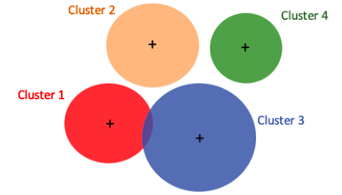
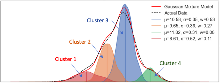
Suppose data points are in four groups as shown in Figure (A.1). There are two or more ways to interpret the data. Figure (A.1) is K-means’ way. It assumes a fixed number of clusters, in this case, four clusters. It then assigns each data point to one cluster. Figure (A.2) is GMM’s way. It assumes a fixed number of Gaussian distributions with varying means and standard deviations. In our case, it assumes four distributions.

I align Figures (A.1) and (A.2) vertically to compare GMM and K-means. GMM describes a data point with the probabilities of coming from four distributions, and K-means identifies a data point to one and only one cluster. Assume a data point at the very left end. K-means will say it belongs to Cluster 1, while GMM may say it has a 90% probability from the red distribution, a 9% probability from the orange distribution, a 0.9% probability from the blue distribution, and a 0.1% probability from the green distribution, or [90%, 9%, 0.9%, 0.1%] chances from the [red, orange, blue, green] distributions. K-Means can be considered a special case of GMM in that the probability of one data point belonging to a cluster is 1, and all other probabilities are 0. Or we can say K-means performs hard classification and Gaussian does soft classification.

(B) What Are the Advantages of GMM over K-means?

While K-Means is a simple and fast clustering method, it may have forced a data point to a cluster but not truly capture the patterns in data. GMM is more intuitive in describing the underlying data patterns. For example, if asked about tomorrow’s weather, we will prudently say ”51% chance hailstorm and 49% rain” and won’t say “definitely 100% hailstorm.”

(C) From Gaussian to GMM

Another motivation to use GMM is when the distributions of instances are multimodal, i.e., there is more than one “peak” in the distribution of data. The multimodal distributions look like a mixture of unimodal distributions. The Gaussian distribution is unimodal and has many nice properties, making it a good choice in the mixture model.

(D) The Problem We Try to Solve

We do not know the probabilities z = [90%, 9%, 0.9%, 0.1%] in GMM, and we do not even know the means µ and the variances ⍴ of each Gaussian distribution. The only thing we know at this moment is that there are four Gaussian distributions. The good news is that the probabilities z, the means µ and variances ⍴ all can be estimated through the Expectation-Maximization algorithm that I am going to present now. With the solution, we can say a data point has [90%, 9%, 0.9%, 0.1%] chances from the four distributions.

If z is known, we can predict a data point x. It is denoted as p(x|z) and is read as “given z, the probability of x is p(x|z).” But what we want to know is the reverse: Given a data point x, what is the distribution that it belongs to. It is denoted as p(z|x) and is read as “give a data point x, the probability that it belongs to z is p(z|x).” I want to remind readers that the conditional probability p(x|z) is not new. It is the essence of any machine learning models. Let’s take a logistic regression Y = a + bX as an example. The a and b are the parameters like z, or z=(a,b). The prediction for Y is “given the parameters a and b, what is the prediction when the value of X is x”, or p(X=x|a,b).

How do we get the p(z|x)? This is what the Bayes’ Theorem is. The relationship between p(z|x) and p(x|z) has been figured out mathematically by an English Presbyterian minister, statistician, and philosopher the Reverend Thomas Bayes (c. 1701–1761).

(E) Use Bayes’ Theorem to Help

The Bayes’ Theorem is shown in Equation (1):

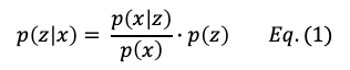
Here p(z) is called the prior probability. It refers to any prior belief or known probability. The p(z|x) is called the posterior probability. It is the probability that takes both prior brief about z, and new data (the new prediction given z) into account. Finally, the ratio p(x|z)/p(x) is called the likelihood ratio. Using these terms, Bayes’ theorem can be rephrased as “the posterior probability equals the prior probability times the likelihood ratio.” A posterior probability can subsequently become a prior for a new updated posterior probability if new information arrives. This iterative process is what the Expectation-Maximization is built on.

(F) How Does GMM Get Its Parameter Estimation?

There are three sets of unknown parameters for estimation: (z, µ, σ). To estimate (µ, σ) in a standard Gaussian distribution, we can use the Maximum log-likelihood Estimation (MLE). You may have learned MLE in linear regression. Now there is one more unknown parameter z, we can first guess any value for z and apply MLE to estimate (µ, σ). Then θ = (µ, σ) is fed back to compute and update z. The updated z is used in MLE to estimate θ = (µ, σ). This iterative process is called the Expectation-Maximization Algorithm. Let me explain more in (F.1) and (F.2).

(F.1) Maximum log-likelihood Estimation (MLE)

I will explain the intuition of MLE by adopting the conventional notations in many textbooks and on-line resources. The conventional notations use the unknown parameter θ that maximizes the likelihood of getting the data we observed.

In a Gaussian distribution, θ is the unknown mean and variance, i.e., θ = (µ, σ). Suppose there are independent and identically distributed (i.i.d.) random samples x1, x2, ⋯, xn, the probability density function (p.d.f) of each xi is f(xi;θ), which means the probability of sample xi in a Gaussian distribution with parameter θ = (µ, σ). The joint probability density function of all observed samples x1, x2, ⋯, xn, is called L(θ):

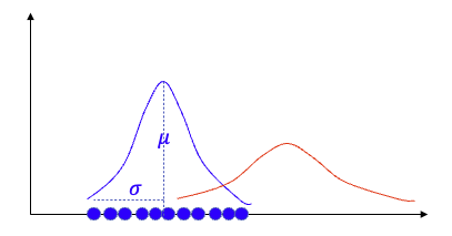
MLE is the algorithm to find the θ that maximizes the above joint density probability. Or we can say MLE finds the optimal θ that these samples are most likely coming from. In Figure (F.1), there are blue dots and all possible Gaussian distributions with their (µ, σ). Which Gaussian distribution is most likelihood that the blue dots coming from? MLE is the algorithm to find (µ, σ).

The second equality in the above equation says the joint density probability can be expressed as the product of individual density functions because of the i.i.d. property. The i.i.d. property is a nice assumption and makes many optimization problems tractable. It means a sample xi is drawn is independent of other samples. In many applications this assumption is not too far off.

Finally, by taking the derivative with respect to (µ, σ) separately and setting each derivative to zero, we can solve for the values (µ, σ).

(F.2) Expectation-Maximization

But if we do not know which of the multiple distributions a data point comes from, the estimation becomes more involved. Even so, we still can use an algorithm called Expectation-Maximization (E-M) to derive the parameters. The EM algorithm uses Bayesian statistics. It has the following two steps (E-M).

The E-step: Assigns an initial “guess” for the probability of a data point belonging to a distribution. Given the guess, the MLE can be formulated. For example, the initial guess for the probabilities that a data point coming from red, orange, blue, and green distributions in Figure (A.2) can be z = (0.25, 0.25, 0.25, 0.25). The probability of a data point belonging to distribution is the posterior probability. The E-step simply plugs in values to Equation (1) to get p(z|x). We know the MLE for a single Gaussian distribution. Because z is known, the MLE of multiple Gaussian distributions is actually the probabilities in z multiplying the MLE of each Gaussian distribution. It is the weighted sum of the MLEs, and the weights are the values in z.

The M-step: This step is the standard MLE to estimate the parameters (µ,⍴). The new parameters are fed to the E-step to assign a posterior probability again. The E-step and M-step will repeat iteratively until convergence.

(G) How Does GMM Define Outlier Score?

GMM outputs the probability of data points to the different Gaussian distributions. This output becomes a natural way to define the outliers. Those data points that have very low fit values are considered outliers. See [2] for the definition. Because other algorithms define high outlier scores for outliers, for consistency, the low fit values are inverted to become high values as the outlier scores.

(H) Modeling procedure

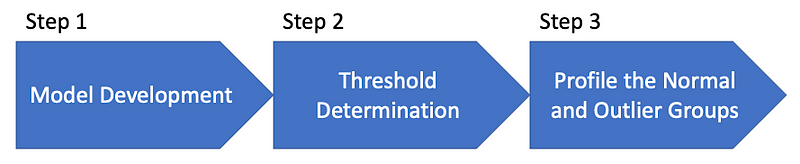
In this book, I apply the following modeling procedure for the model development, assessment, and interpretation of the results.

1. Model development
2. Threshold determination
3. Descriptive statistics of the normal and abnormal groups

With the outlier scores, you will choose a threshold to separate the abnormal observations with high outlier scores from normal observations. If any prior knowledge suggests the percentage of anomalies should be no more than 1%, you can choose a threshold that results in approximately 1% of anomalies.

The descriptive statistics (such as the means and standard deviations) of the features between the two groups are important to communicate the soundness of the model. If it is expected that the mean of a feature in the abnormal group is higher than that of the normal group, it will be counter-intuitive if the result is the opposite. In such a case, you shall investigate, modify, or drop the feature and do modeling again.

(H.1) Step 1 — Build your Model

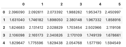
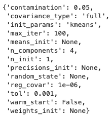
Like before, I will use the utility function generate_data() of PyOD to generate ten percent outliers. To make the case more interesting, the data generation process (DGP) will create six variables. Although this mock dataset has the target variable Y, the unsupervised models only use the X variables. The Y variable is simply for validation. I set the percentage of outliers to 5% with “contamination=0.05.”

The first five records of the six variables look like the following:

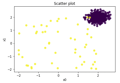
Let me just plot the first two variables in a scatter plot. The yellow points in the scatterplot are the ten percent outliers. The normal observations are the purple points.

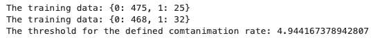
It is fairly easy to build a model with PyOD, thanks to its unified APIs. Below we declare and fit the model, then use the function decision_functions() to generate the outlier scores for the training and test data.

The parameter contamination=0.05 declares a contamination rate of 5%. The contamination rate is the percentage of outliers. In most cases, we do not know the percentage of outliers so we can assign a value based on any prior knowledge. PyOD defaults the contamination rate to 10%. This parameter does not affect the calculation of the outlier scores. PyOD uses it to derive the threshold for the outlier scores and applies the function predict() to assign the labels (1 or 0). I made a short function count_stat() in the code below to show the count of predicted “1” and “0” values. The syntax .threshold_ shows the threshold at the assigned contamination rate. Any outlier score higher than the threshold is considered an outlier.

(H.2) Step 2 — Determine a reasonable threshold

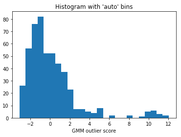
In most cases, we do not know the percentage of outliers. We can use the histogram of the outlier score to select a reasonable threshold value. The threshold determines the size of the abnormal group. If any prior knowledge suggests the percentage of anomalies should be no more than 1%, you can choose a threshold that results in approximately 1% of anomalies. Figure (H.2) presents the histogram of the outlier score. It appears we can set the threshold at 200.0 because there is a natural cut in the histogram. If we select a low value for the threshold, the count of outliers will be high, and vice versa.

(H.3) Step 3 — Present the summary statistics of the normal and the abnormal groups

As explained in Chapter 1, the descriptive statistics (such as the means and standard deviations) of the features between the two groups are important to demonstrate the soundness of a model. I create a short function descriptive_stat_threshold() to show the sizes and descriptive statistics of the features for the normal and the outlier groups based on the threshold. Below I simply use the threshold at 5%. You can test a range of thresholds for a reasonable size for the outlier group.

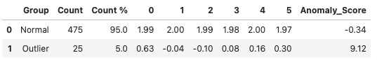
The above table presents the characteristics of the normal and abnormal groups. It shows the count and count percentage of the normal and outlier groups. The “Anomalous_Score” is the average anomaly score. You are reminded to label the features with their feature names for an effective presentation. The table tells us several important results:

• The size of the outlier group: The outlier group is about 5%. Remember the size of the outlier group is determined by the threshold. If you choose a higher value for the threshold, the size will shrink.
• The average anomaly score: The average outlier score of the outlier group is far higher than that of the normal group (9.12>-0.34). You do not need to interpret too much on the scores.
• The feature statistics in each group: The above shows the means of the features in the outlier group are smaller than those of the normal group. Whether the means of the features in the outlier group should be higher or lower depends on business applications. It is important that all the means should be consistent with the domain knowledge.

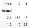
Because we have the ground truth in our data generation, we can produce a confusion matrix to understand the model performance. The model delivers a decent job and identifies all 25 outliers.

(I) Achieve Model Stability by Aggregating Multiple Models

Distribution-based methods can be very susceptible to noise and overfitting in the training data. GMM assumes a specific distribution of the data and then tries to learn the parameters of this distribution. If the assumption for the distribution is inaccurate (not Gaussian), the data will not fit the model well and the model will produce many outliers. Also, if one assumes too many underlying Gaussian distributions (number of mixture components), it tends to overfit the data.

An overfitted model produces an unstable outcome. The solution is to train the models with a range of hyperparameters and then aggregate the scores. The chance of overfitting will be greatly reduced and the prediction accuracy will be improved.

In order not to assume a large number of mixture components, I produce seven GMM models for a range of clusters. The average prediction of these models will be the final model prediction.

The predictions are normalized and stored in the data frame “train_scores_norm”. The PyOD module offers four aggregation methods and you only need to use one method to produce the outcome.

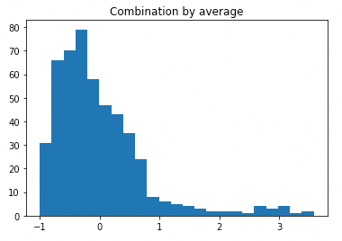
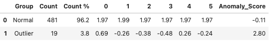
Figure (I) plots the histogram of the outlier score. It suggests 2.0 to be the threshold. Then I generate the descriptive statistics table in Table (I). It identifies 19 data points to be the outliers. Readers shall apply similar interpretations to Table (H.3).

(J) Summary of the GMM Algorithm

• GMM describes a data point with the probabilities of coming from different distributions, and K-means identifies a data point to one and only one cluster.
• The conditional probability p(z|x) is read as “give a data point x, the probability that it belongs to z is p(z|x).” By using the Bayes’ Theorem, we can get the posterior probability p(z|x).
• GMM uses Expectation-Maximization to find the optimal value for the posterior probability p(z|x). The E-step assigns an initial “guess” for the probability of a data point belonging to a distribution. Given the guess, the MLE can be formulated. The M-step is the standard MLE to estimate the parameters. The new parameters are fed to the E-step to assign a posterior probability again. The E-step and M-step will repeat iteratively until convergence.
• Those data points that have low fit values to the underlying Gaussian distributions are considered outliers.

(K) Python Notebook: Click here for the notebook

References

• [1] Duda, R. O. & Hart, P. E. (1973), Pattern Classification and Scene Analysis, Wiley, New York
• [2] Charu C. Aggarwal. 2016. Outlier Analysis (2nd. ed.). Springer Publishing Company, Incorporated.

For easy navigation to chapters, I list the chapters at the end.

• Chapter 1 — Introduction
• Chapter 2 — Histogram-Based Outlier Score (HBOS)
• Chapter 3 — Empirical Cumulative Outlier Detection (ECOD)
• Chapter 4 — Isolation Forest (IForest)
• Chapter 5 — Principal Component Analysis (PCA)
• Chapter 6 — One-Class Support Vector Machine (OCSVM)
• Chapter 7 — Gaussian Mixed Models (GMM)
• Chapter 8 — K-nearest Neighbors (KNN)
• Chapter 9 — Local Outlier Factor (LOF)
• Chapter 10 — Clustering-Based Local Outlier Factor (CBLOF)
• Chapter 11 — Extreme Boosting-Based Outlier Detection (XGBOD)
• Chapter 12 — Autoencoders
• Chapter 13 — Under-sampling for Extremely Imbalanced Data
• Chapter 14 — Over-sampling for Extremely Imbalanced Data

Readers are recommended to purchase books by Chris Kuo:

• The explainable AI: https://a.co/d/cNL8Hu4
• Transfer learning for image classification: https://a.co/d/hLdCkMH
• Modern time series anomaly detection: https://a.co/d/ieIbAxM
• Handbook of Anomaly Detection: https://a.co/d/5sKS8bI