Exploring OpenAI Point·E With Jupyter Notebook, VSCode, and Colab

Generate 3D models based on descriptions

Introduction

Point·E is another OpenAI product. While DALL·E generates 2D images, Point·E generates 3D models. It is a system for generating 3D point clouds from prompts, where a point cloud is a discrete set of data points in space. 3D models are visual representations of point clouds.

Point·E first generates a single synthetic view using a text-to-image diffusion model, and then produces a 3D point cloud using a second diffusion model which is conditioned on the generated image. To produce a 3D model, it takes only 1–2 minutes on a single GPU. On December 2022, OpenAI released the pre-trained point cloud diffusion models, as well as evaluation code and models.

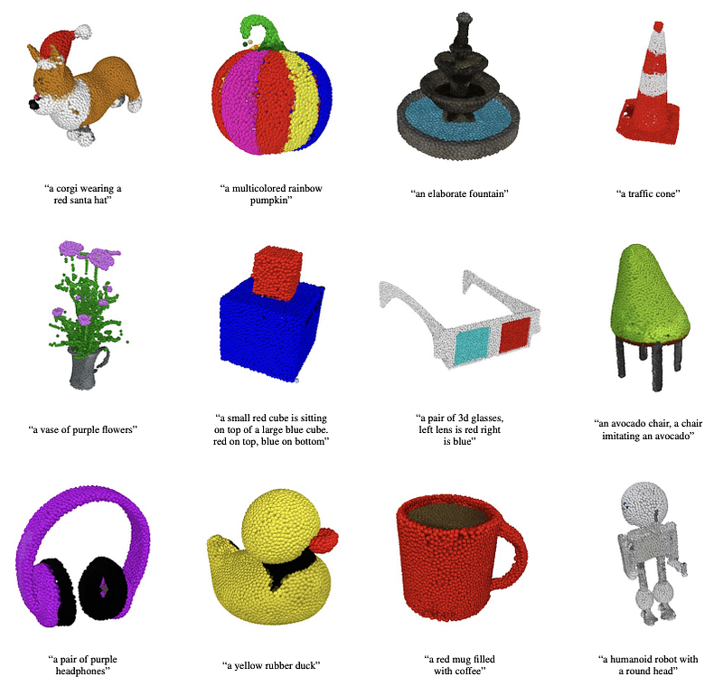
Here are examples of generated 3D models from prompts:

Point·E Demo on Hugging Face

Hugging Face is an American company that develops tools to build applications using machine learning. It was founded in 2016 by Clément Delangue, Julien Chaumond, and Thomas Wolf, originally as a company that developed a chatbot app targeted at teenagers. After open-sourcing the model behind the chatbot, the company becomes the AI community to build, train, and deploy state of the art models powered by referencing open source in machine learning.

Point-E demo: text to 3D is one of the models on Hugging Face. It generates 3D point clouds with Point·E. The demo uses a small, worse quality text-to-3D model to produce 3D point clouds directly from text descriptions.

We use the prompt, 'a colorful flower', to generate a 3D model:

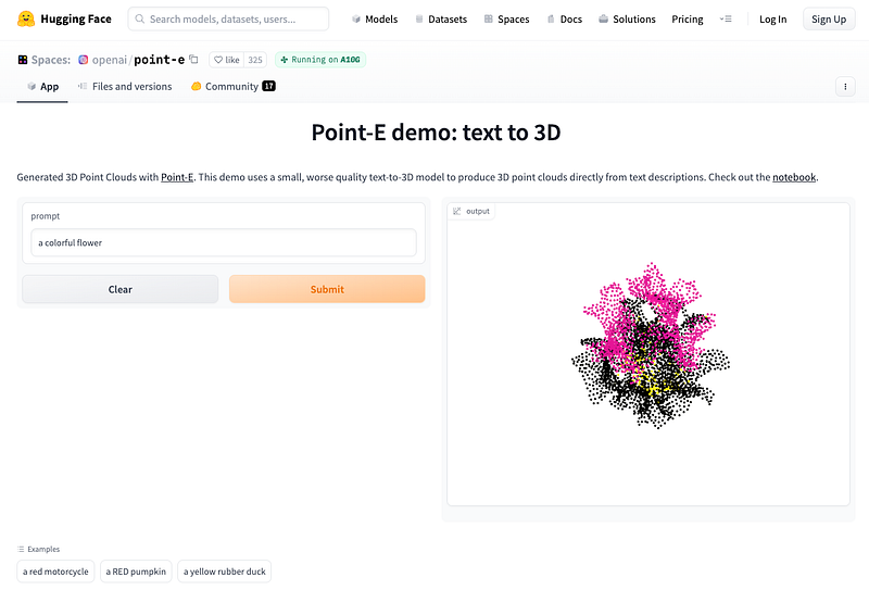
The generated model is displayed using plotly.js, and the following image shows how the 3D model moves with a dragging mouse.

Point·E Demo Repository

Point·E code is open sourced on Github. We follow the instruction to clone the repository and install it:

% git clone https://github.com/openai/point-e.git
% cd point-e
% pip install -e .

The repository provides three examples:

• text2pointcloud.ipynb: Convert text to 3D point cloud.
• image2pointcloud.ipynb: Convert image to 3D point cloud.
• pointcloud2mesh.ipynb: Convert 3D point cloud to a mesh file.

.ipynb stands for Interactive PYthon NoteBook. In order to run these examples, we need to set up notebook working environment. We are going to show Point·E Demo in three working environments — Jupyter Notebook, Visual Studio Code, and Google Colaboratory.

Jupyter Notebook Working Environment

Jupyter Notebook is a web-based interactive computational environment for creating notebook documents. It is built using several open-source libraries, including IPython, ZeroMQ, Tornado, jQuery, Bootstrap, and MathJax. A Jupyter Notebook application is a browser-based language shell, and its core languages are Julia, Python, and R.

There are various ways to view and execute notebook files. The traditional way is to install notebook and ipywidgets with Python 3:

% pip install notebook
% pip install ipywidgets

Then, execute the following command to start a Jupyter server:

% jupyter notebook

It launches the Jupyter Notebook application on the browser. By default, it shows the current directory.

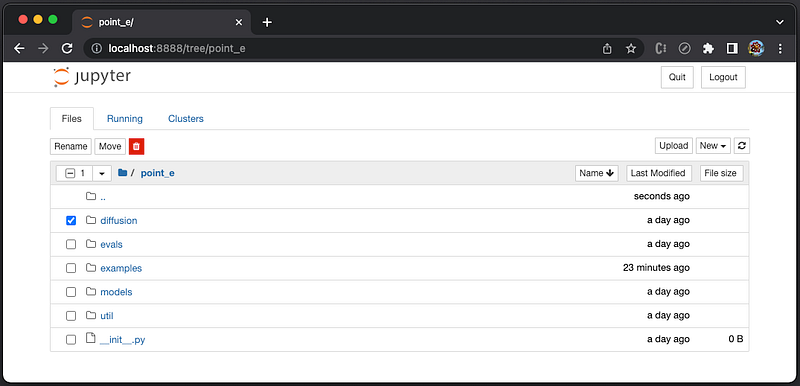
Click New → Python 3, and it launches a new Notebook shell (tab).

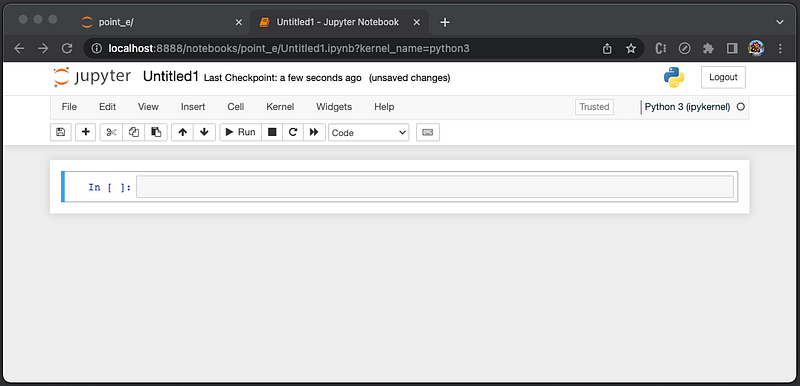
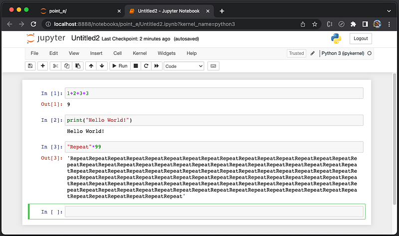
The shell includes an ordered list of input/output cells which can contain code, text, mathematics, plots, and rich media.

Type the mathematics equation, 1+2+3+3, in the input cell, and click Run to execute the code. The output cell displays the result.

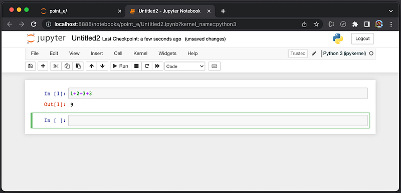
Jupyter Notebook numbers each executed cell based on its execution order. An executing cell is labeled as [*], and unexecuted cell is labeled as [ ]. The same cell can be executed multiple times, and each execution increases the number.

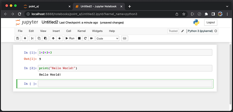
Type a function, print("Hello World!"), in the input cell, and click Run to execute the code. The output cell shows Hello World!.

Type "Repeat"*99 in the input cell, and click Run to execute the code. The output cell shows a new string with "Repeat" being repeated 99 times.

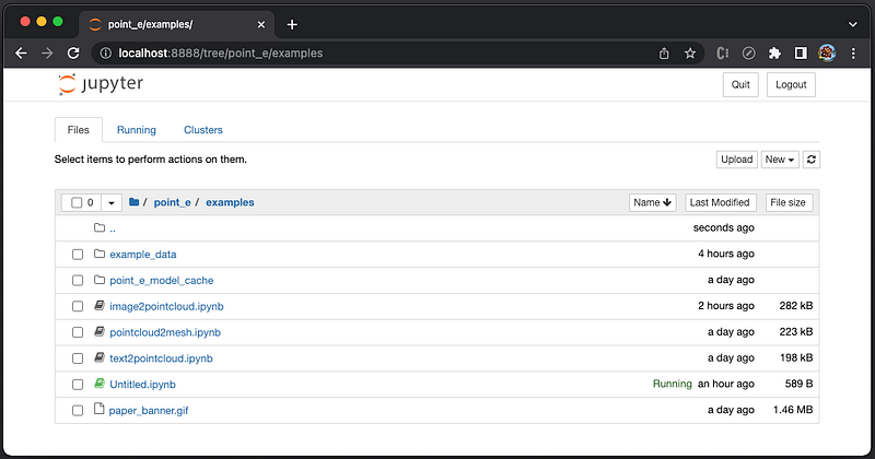
Now we are ready to explore Point·E examples, located at http://localhost:8888/tree/point_e/examples.

text2pointcloud.ipynb

This is a text-to-model example that takes a text description, generates 3D point cloud, and displays a 3D model. This model has limited capabilities, but it does understand some simple categories and colors.

Here is the source code of point_e/examples/text2pointcloud.ipynb:

{
 "cells": [
  {
   "cell_type": "code",
   "execution_count": null,
   "metadata": {},
   "outputs": [],
   "source": [
    "import torch\n",
    "from tqdm.auto import tqdm\n",
    "\n",
    "from point_e.diffusion.configs import DIFFUSION_CONFIGS, diffusion_from_config\n",
    "from point_e.diffusion.sampler import PointCloudSampler\n",
    "from point_e.models.download import load_checkpoint\n",
    "from point_e.models.configs import MODEL_CONFIGS, model_from_config\n",
    "from point_e.util.plotting import plot_point_cloud"
   ]
  },
  {
   "cell_type": "code",
   "execution_count": null,
   "metadata": {},
   "outputs": [],
   "source": [
    "device = torch.device('cuda' if torch.cuda.is_available() else 'cpu')\n",
    "\n",
    "print('creating base model...')\n",
    "base_name = 'base40M-textvec'\n",
    "base_model = model_from_config(MODEL_CONFIGS[base_name], device)\n",
    "base_model.eval()\n",
    "base_diffusion = diffusion_from_config(DIFFUSION_CONFIGS[base_name])\n",
    "\n",
    "print('creating upsample model...')\n",
    "upsampler_model = model_from_config(MODEL_CONFIGS['upsample'], device)\n",
    "upsampler_model.eval()\n",
    "upsampler_diffusion = diffusion_from_config(DIFFUSION_CONFIGS['upsample'])\n",
    "\n",
    "print('downloading base checkpoint...')\n",
    "base_model.load_state_dict(load_checkpoint(base_name, device))\n",
    "\n",
    "print('downloading upsampler checkpoint...')\n",
    "upsampler_model.load_state_dict(load_checkpoint('upsample', device))"
   ]
  },
  {
   "cell_type": "code",
   "execution_count": null,
   "metadata": {},
   "outputs": [],
   "source": [
    "sampler = PointCloudSampler(\n",
    "    device=device,\n",
    "    models=[base_model, upsampler_model],\n",
    "    diffusions=[base_diffusion, upsampler_diffusion],\n",
    "    num_points=[1024, 4096 - 1024],\n",
    "    aux_channels=['R', 'G', 'B'],\n",
    "    guidance_scale=[3.0, 0.0],\n",
    "    model_kwargs_key_filter=('texts', ''), # Do not condition the upsampler at all\n",
    ")"
   ]
  },
  {
   "cell_type": "code",
   "execution_count": null,
   "metadata": {},
   "outputs": [],
   "source": [
    "# Set a prompt to condition on.\n",
    "prompt = 'a red motorcycle'\n",
    "\n",
    "# Produce a sample from the model.\n",
    "samples = None\n",
    "for x in tqdm(sampler.sample_batch_progressive(batch_size=1, model_kwargs=dict(texts=[prompt]))):\n",
    "    samples = x"
   ]
  },
  {
   "cell_type": "code",
   "execution_count": null,
   "metadata": {},
   "outputs": [],
   "source": [
    "pc = sampler.output_to_point_clouds(samples)[0]\n",
    "fig = plot_point_cloud(pc, grid_size=3, fixed_bounds=((-0.75, -0.75, -0.75),(0.75, 0.75, 0.75)))"
   ]
  }
 ],
 "metadata": {
  "kernelspec": {
   "display_name": "Python 3.9.9 64-bit ('3.9.9')",
   "language": "python",
   "name": "python3"
  },
  "language_info": {
   "codemirror_mode": {
    "name": "ipython",
    "version": 3
   },
   "file_extension": ".py",
   "mimetype": "text/x-python",
   "name": "python",
   "nbconvert_exporter": "python",
   "pygments_lexer": "ipython3",
   "version": "3.9.9 (main, Aug 15 2022, 16:40:41) \n[Clang 13.1.6 (clang-1316.0.21.2.5)]"
  },
  "orig_nbformat": 4,
  "vscode": {
   "interpreter": {
    "hash": "b270b0f43bc427bcab7703c037711644cc480aac7c1cc8d2940cfaf0b447ee2e"
   }
  }
 },
 "nbformat": 4,
 "nbformat_minor": 2
}

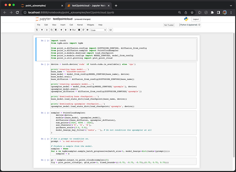
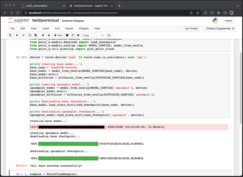
At http://localhost:8888/tree/point_e/examples, click on text2pointcloud.ipynb. It launches a new shell (tab) that shows 5 cells of the file, and the first cell is active.

Execute the first cell [1], and it imports packages. The next cell becomes active.

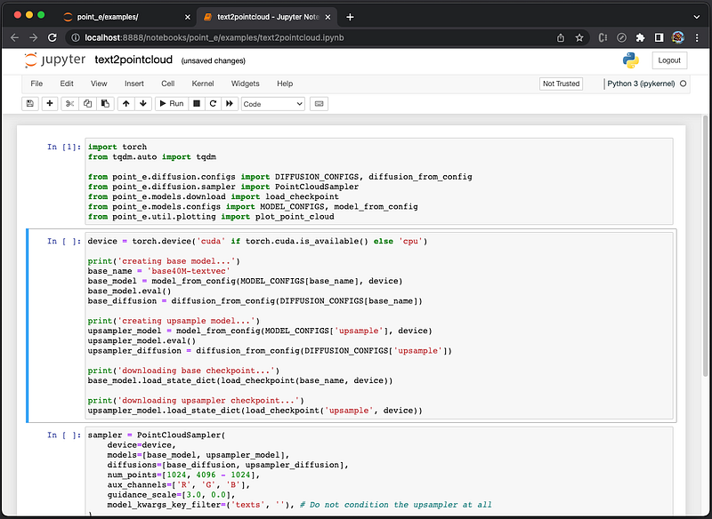
Execute the second cell [2]. It creates base model and upsample model, downloads base checkpoint and upsampler checkpoint. The output shows <All keys matched successfully>. The next cell becomes active.

Execute the third cell [3]. It creates point cloud sampler with specified parameters. The next cell becomes active.

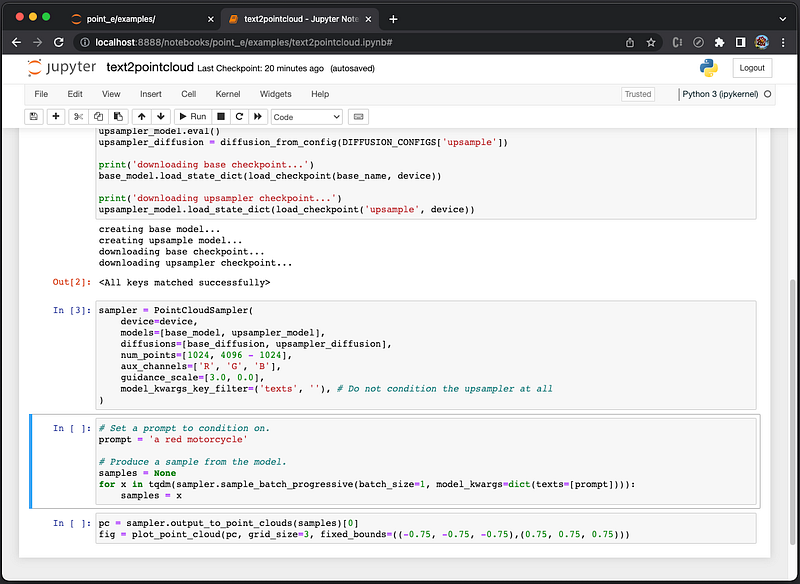
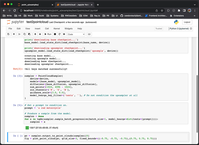
The fourth cell uses the prompt, 'a red motorcycle'. Execute the cell [5], and it creates point cloud sampler (It took 37 minutes and 55 seconds on a MacBook Pro to finish this step). The next cell becomes active.

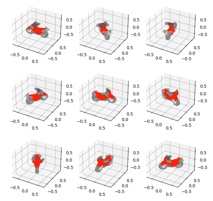
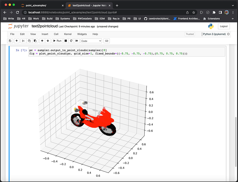
The fifth cell displays the point cloud sampler in 3D. Execute the cell [6], and it shows a 3D model in 3x3 grids.

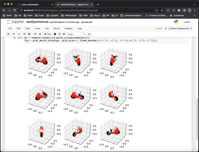
It is slightly different from the 3D model displayed as the article’s head image, since AI generated result is not deterministic.

Change to grid_size=1, and re-execute the cell. The fifth cell [7] shows 3D model in 1x1 grid.

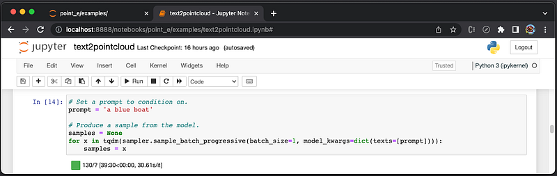
Go back to the fourth cell, and change the prompt to 'a blue boat'. Execute it, and the cell number increases to 14 after a few tries.

Execute the fifth cell [15], and it shows a 3D model in 3x3 grids of a blue boat.

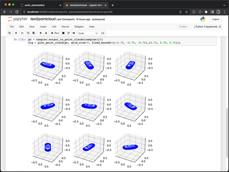
image2pointcloud.ipynb

This is an image-to-model example that takes an image, generates 3D point cloud, and displays a 3D model.

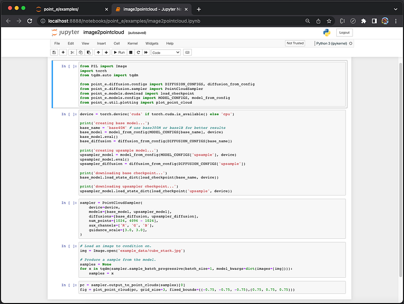
Here is the source code of point_e/examples/image2pointcloud.ipynb:

{
 "cells": [
  {
   "cell_type": "code",
   "execution_count": null,
   "metadata": {},
   "outputs": [],
   "source": [
    "from PIL import Image\n",
    "import torch\n",
    "from tqdm.auto import tqdm\n",
    "\n",
    "from point_e.diffusion.configs import DIFFUSION_CONFIGS, diffusion_from_config\n",
    "from point_e.diffusion.sampler import PointCloudSampler\n",
    "from point_e.models.download import load_checkpoint\n",
    "from point_e.models.configs import MODEL_CONFIGS, model_from_config\n",
    "from point_e.util.plotting import plot_point_cloud"
   ]
  },
  {
   "cell_type": "code",
   "execution_count": null,
   "metadata": {},
   "outputs": [],
   "source": [
    "device = torch.device('cuda' if torch.cuda.is_available() else 'cpu')\n",
    "\n",
    "print('creating base model...')\n",
    "base_name = 'base40M' # use base300M or base1B for better results\n",
    "base_model = model_from_config(MODEL_CONFIGS[base_name], device)\n",
    "base_model.eval()\n",
    "base_diffusion = diffusion_from_config(DIFFUSION_CONFIGS[base_name])\n",
    "\n",
    "print('creating upsample model...')\n",
    "upsampler_model = model_from_config(MODEL_CONFIGS['upsample'], device)\n",
    "upsampler_model.eval()\n",
    "upsampler_diffusion = diffusion_from_config(DIFFUSION_CONFIGS['upsample'])\n",
    "\n",
    "print('downloading base checkpoint...')\n",
    "base_model.load_state_dict(load_checkpoint(base_name, device))\n",
    "\n",
    "print('downloading upsampler checkpoint...')\n",
    "upsampler_model.load_state_dict(load_checkpoint('upsample', device))"
   ]
  },
  {
   "cell_type": "code",
   "execution_count": null,
   "metadata": {},
   "outputs": [],
   "source": [
    "sampler = PointCloudSampler(\n",
    "    device=device,\n",
    "    models=[base_model, upsampler_model],\n",
    "    diffusions=[base_diffusion, upsampler_diffusion],\n",
    "    num_points=[1024, 4096 - 1024],\n",
    "    aux_channels=['R', 'G', 'B'],\n",
    "    guidance_scale=[3.0, 3.0],\n",
    ")"
   ]
  },
  {
   "cell_type": "code",
   "execution_count": null,
   "metadata": {},
   "outputs": [],
   "source": [
    "# Load an image to condition on.\n",
    "img = Image.open('example_data/cube_stack.jpg')\n",
    "\n",
    "# Produce a sample from the model.\n",
    "samples = None\n",
    "for x in tqdm(sampler.sample_batch_progressive(batch_size=1, model_kwargs=dict(images=[img]))):\n",
    "    samples = x"
   ]
  },
  {
   "cell_type": "code",
   "execution_count": null,
   "metadata": {},
   "outputs": [],
   "source": [
    "pc = sampler.output_to_point_clouds(samples)[0]\n",
    "fig = plot_point_cloud(pc, grid_size=3, fixed_bounds=((-0.75, -0.75, -0.75),(0.75, 0.75, 0.75)))"
   ]
  }
 ],
 "metadata": {
  "kernelspec": {
   "display_name": "Python 3.9.9 64-bit ('3.9.9')",
   "language": "python",
   "name": "python3"
  },
  "language_info": {
   "codemirror_mode": {
    "name": "ipython",
    "version": 3
   },
   "file_extension": ".py",
   "mimetype": "text/x-python",
   "name": "python",
   "nbconvert_exporter": "python",
   "pygments_lexer": "ipython3",
   "version": "3.9.9"
  },
  "orig_nbformat": 4,
  "vscode": {
   "interpreter": {
    "hash": "b270b0f43bc427bcab7703c037711644cc480aac7c1cc8d2940cfaf0b447ee2e"
   }
  }
 },
 "nbformat": 4,
 "nbformat_minor": 2
}

At http://localhost:8888/tree/point_e/examples, click on image2pointcloud.ipynb. It launches a new shell (tab) that shows 5 cells of the file, and the first cell is active.

Execute the first cell [1], and it imports packages. The next cell becomes active.

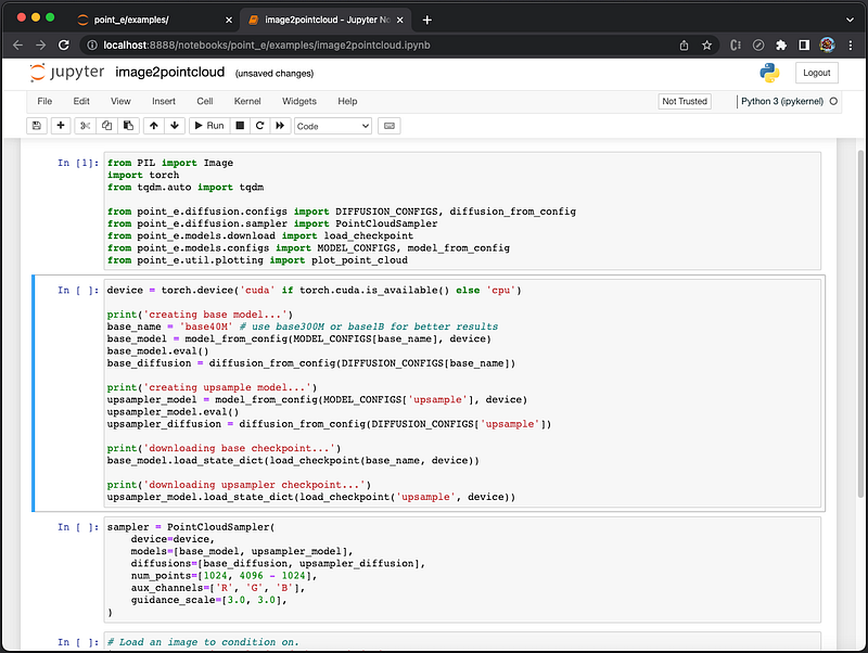
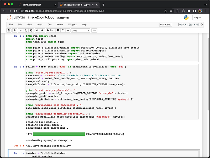
Execute the second cell [2]. It creates base model and upsample model, downloads base checkpoint and upsampler checkpoint. The output shows <All keys matched successfully>. The next cell becomes active.

Execute the third cell [3]. It creates point cloud sampler with specified parameters. The next cell becomes active.

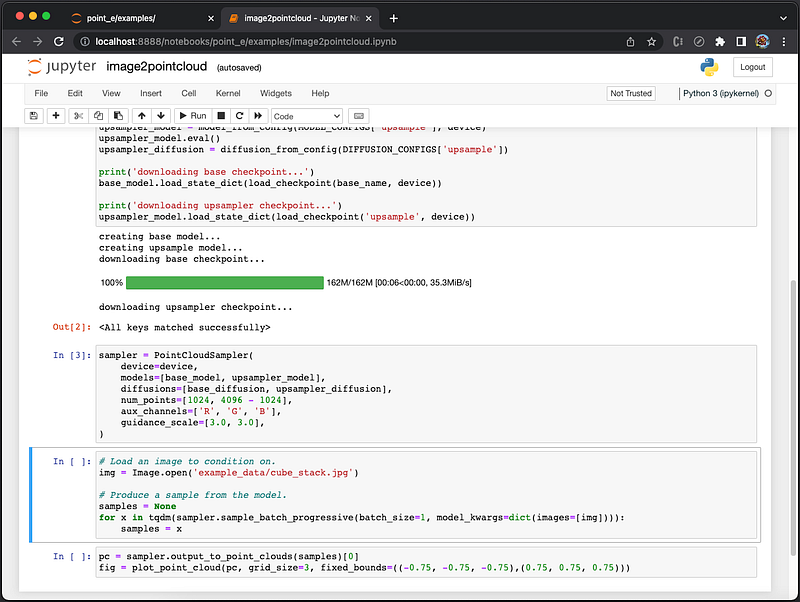
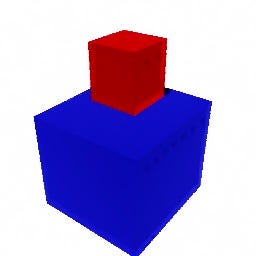
The fourth cell uses the provided image, 'example_data/cube_stack.jpg'.

Execute the cell [4], and it creates point cloud sampler (It took 58 minutes and 46 seconds on a MacBook Pro to finish this step). The next cell becomes active.

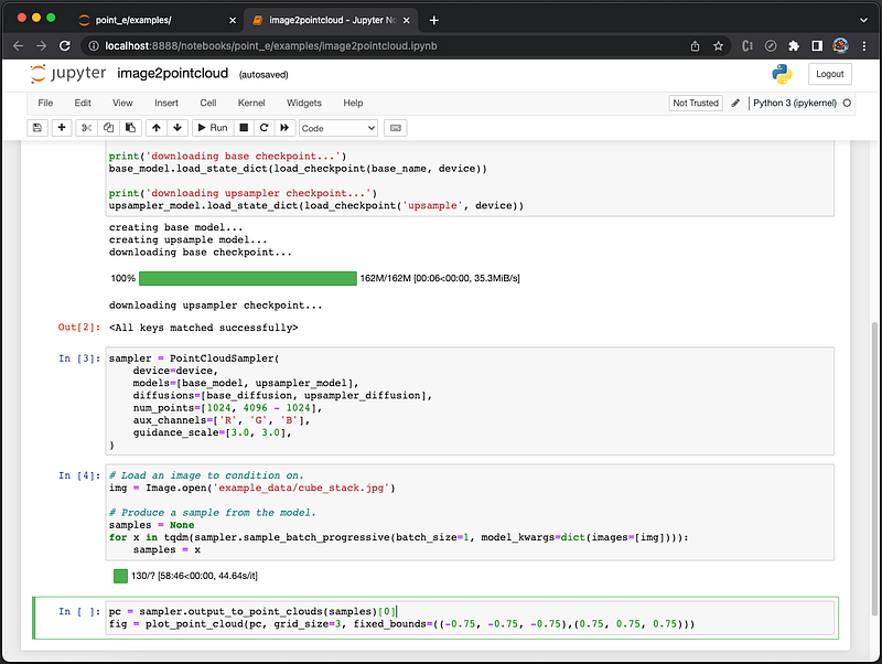
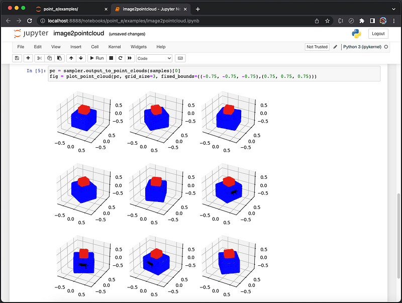
The fifth cell [5] displays point cloud in 3D. Execute the cell, and it shows a 3D model in 3x3 grids.

We can also use our own image to generate a 3D model. Name this file as fireHydrant.jpg under the folder example_data.

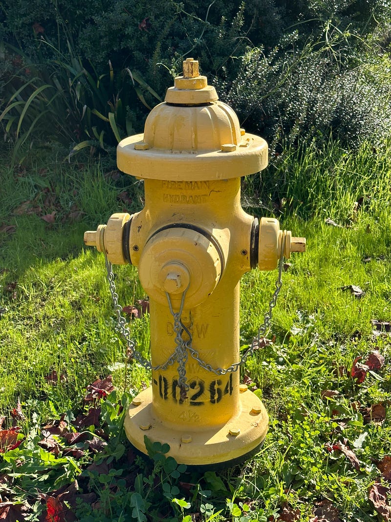
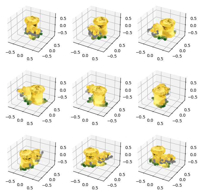
Go back to the fourth cell, and change the image name to 'example_data/fireHydrant.jpg'. After executing the fourth and fifth cells, it shows a 3D model in 3x3 grids of a yellow fire hydrant.

pointcloud2mesh.ipynb

This is an example that converts a 3D point cloud file to a mesh file.

Here is the source code of point_e/examples/pointcloud2mesh.ipynb:

{
 "cells": [
  {
   "cell_type": "code",
   "execution_count": null,
   "metadata": {},
   "outputs": [],
   "source": [
    "from PIL import Image\n",
    "import torch\n",
    "import matplotlib.pyplot as plt\n",
    "from tqdm.auto import tqdm\n",
    "\n",
    "from point_e.models.download import load_checkpoint\n",
    "from point_e.models.configs import MODEL_CONFIGS, model_from_config\n",
    "from point_e.util.pc_to_mesh import marching_cubes_mesh\n",
    "from point_e.util.plotting import plot_point_cloud\n",
    "from point_e.util.point_cloud import PointCloud"
   ]
  },
  {
   "cell_type": "code",
   "execution_count": null,
   "metadata": {},
   "outputs": [],
   "source": [
    "device = torch.device('cuda' if torch.cuda.is_available() else 'cpu')\n",
    "\n",
    "print('creating SDF model...')\n",
    "name = 'sdf'\n",
    "model = model_from_config(MODEL_CONFIGS[name], device)\n",
    "model.eval()\n",
    "\n",
    "print('loading SDF model...')\n",
    "model.load_state_dict(load_checkpoint(name, device))"
   ]
  },
  {
   "cell_type": "code",
   "execution_count": null,
   "metadata": {},
   "outputs": [],
   "source": [
    "# Load a point cloud we want to convert into a mesh.\n",
    "pc = PointCloud.load('example_data/pc_corgi.npz')\n",
    "\n",
    "# Plot the point cloud as a sanity check.\n",
    "fig = plot_point_cloud(pc, grid_size=2)"
   ]
  },
  {
   "cell_type": "code",
   "execution_count": null,
   "metadata": {},
   "outputs": [],
   "source": [
    "# Produce a mesh (with vertex colors)\n",
    "mesh = marching_cubes_mesh(\n",
    "    pc=pc,\n",
    "    model=model,\n",
    "    batch_size=4096,\n",
    "    grid_size=32, # increase to 128 for resolution used in evals\n",
    "    progress=True,\n",
    ")"
   ]
  },
  {
   "cell_type": "code",
   "execution_count": null,
   "metadata": {},
   "outputs": [],
   "source": [
    "# Write the mesh to a PLY file to import into some other program.\n",
    "with open('mesh.ply', 'wb') as f:\n",
    "    mesh.write_ply(f)"
   ]
  }
 ],
 "metadata": {
  "kernelspec": {
   "display_name": "Python 3.9.9 64-bit ('3.9.9')",
   "language": "python",
   "name": "python3"
  },
  "language_info": {
   "codemirror_mode": {
    "name": "ipython",
    "version": 3
   },
   "file_extension": ".py",
   "mimetype": "text/x-python",
   "name": "python",
   "nbconvert_exporter": "python",
   "pygments_lexer": "ipython3",
   "version": "3.9.9"
  },
  "orig_nbformat": 4,
  "vscode": {
   "interpreter": {
    "hash": "b270b0f43bc427bcab7703c037711644cc480aac7c1cc8d2940cfaf0b447ee2e"
   }
  }
 },
 "nbformat": 4,
 "nbformat_minor": 2
}

At http://localhost:8888/tree/point_e/examples, click on pointcloud2mesh.ipynb. It launches a new shell (tab) that shows 5 cells of the file, and the first cell is active.

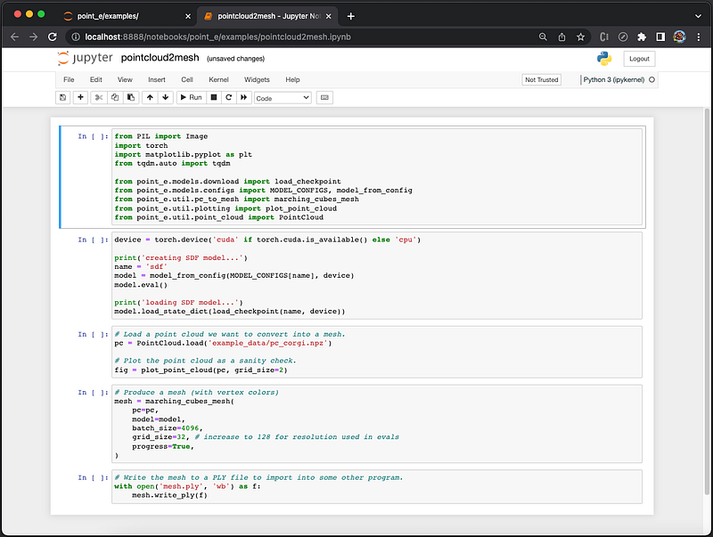
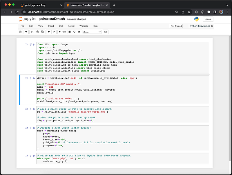
Execute the first cell [1], and it imports packages. The next cell becomes active.

Execute the second cell [2]. It creates and loads SDF model. The output shows <All keys matched successfully>. The next cell becomes active.

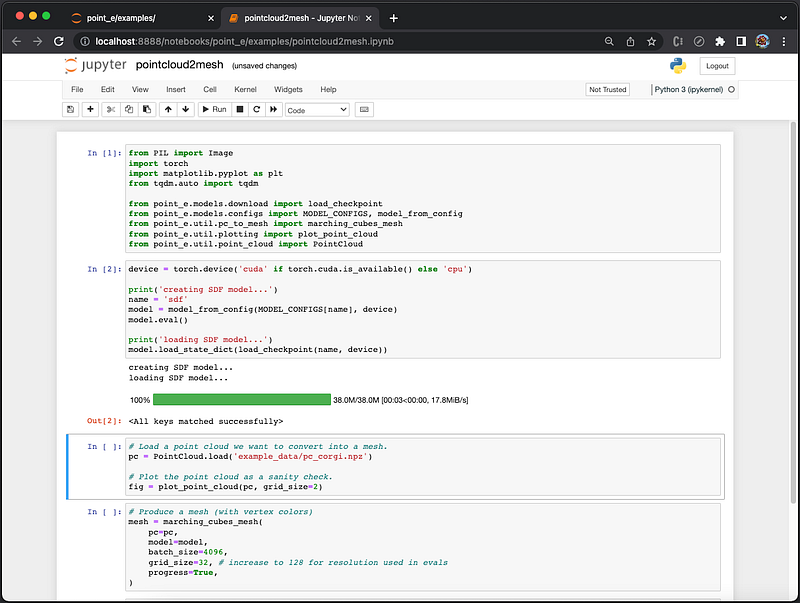
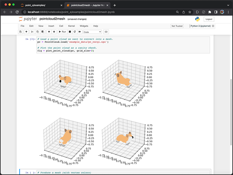
The third cell loads a 3D point cloud file, 'example_data/pc_corgi.npz'.

NumPy is a Python library that provides a multidimensional array object, various derived objects, and an assortment of routines for fast operations on arrays.

• .npz is a zip file containing multiple .npy files, one for each array.
• .npy is NumPy’s standard binary file for persisting a single arbitrary NumPy array on disk. The format stores all of the shape and dtype information necessary to reconstruct the array correctly even on another machine with a different architecture.

Execute the third cell [3]. It loads point cloud sampler, and verifies that data is valid for a 3D model in 2x2 grids. The next cell becomes active.

Execute the four cell [4]. It produces a mesh with vertex colors, and the next cell becomes active.

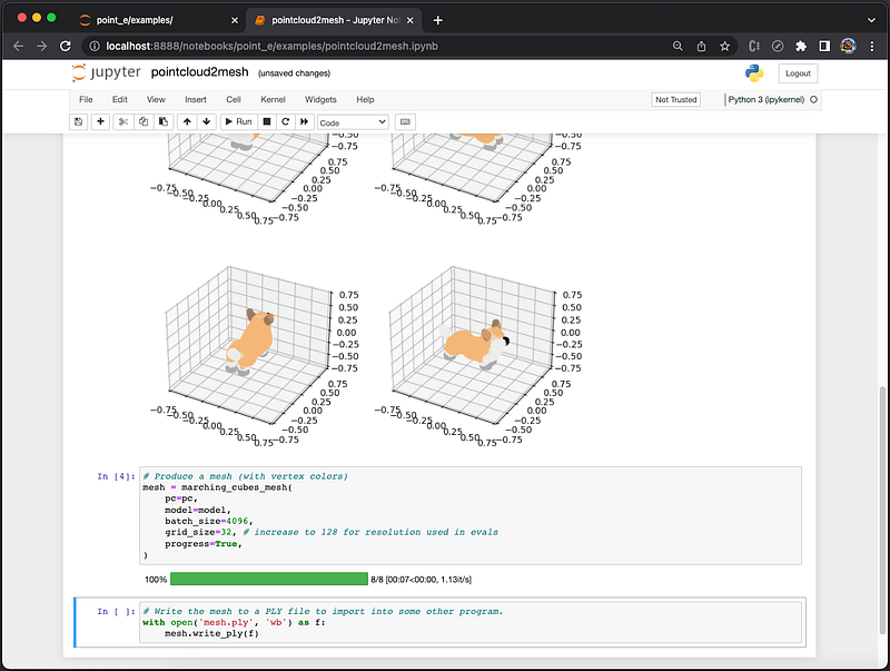
The fifth cell produces a .fly file, in the Polygon File Format or the Stanford Triangle Format. It was principally designed to store 3D data. There are two versions of the file format, one in ASCII and the other one in binary.

Execute the cell [5], and it creates mesh.ply:

ply
format binary_little_endian 1.0
element vertex 1585
property float x
property float y
property float z
property uchar red
property uchar green
property uchar blue
element face 3170
property list uchar int vertex_index
end_header
HO��1��8�����8���1��(� ����8���<��8�����8��c���������B�!��1��������8���0���v������ ��1���v�����8��;r��H(J���ߔ9��1��H(J����8���1��@ ����X���1���1�>��g8���1��2�>��e8������1�>ѝo8�� t���
�>ҝn�(��1���
...

• ply: It is the header that starts with the magic number, ply.
• format: It indicates which variation of the PLY format. Obviously, this file is in binary format.
• First group of element and property: It describes that there are 1585 vertices, each represented as a point of (x, y, z, red, green, blue), where x, y, z are float, and red, green, blue are uchar.
• Second group of element and property: It describes that there are 3170 polygonal faces, where vertex_index is a list, whose number of entries is a uchar, and each list entry is an int.
• end_header: It indicates the end of the header.

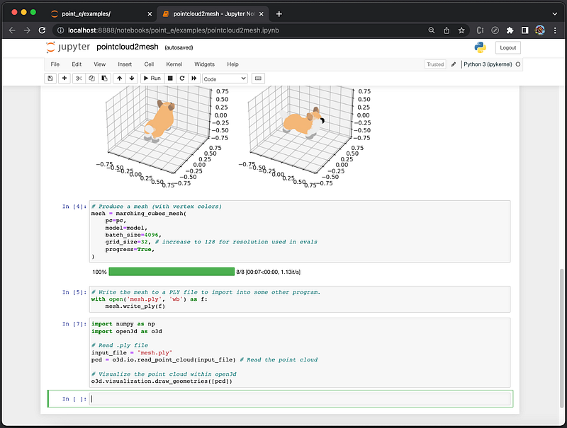
The official example ends with mesh.ply, and the next active cell is empty.

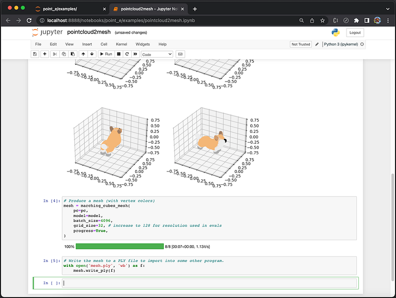
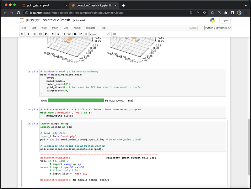
We add code in the empty cell to display the generated mesh.ply:

import numpy as np
import open3d as o3d

# Read .ply file
input_file = "mesh.ply"
pcd = o3d.io.read_point_cloud(input_file) # Read the point cloud

# Visualize the point cloud within open3d
o3d.visualization.draw_geometries([pcd]) 

Execute the cell [6], and it shows ModuleNotFoundError about open3d.

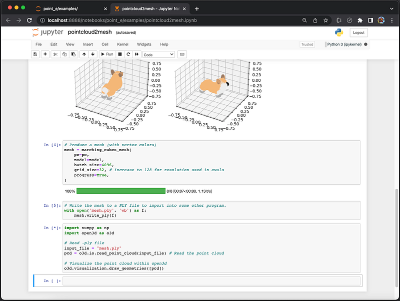
Install open3d to resolve the issue:

% pip install open3d

Execute the cell again, and it is in the executing state [*].

There is a popup window of Open3D that shows a corgi. Here is how the 3D model moves with a dragging mouse.

Upon exiting this Open3D window, the cell finishes execution and numbers the cell 7.

Visual Studio Code Working Environment

We have used Jupyter Notebook to execute notebook files. They can be executed by Visual Studio Code (VSCode) as well.

Open the project in VSCode, and all code are available for viewing, including the folders of .ipynb_checkpoints and point_e_model_cache.

Open point_e/examples/pointcloud2mesh.ipynb in the Editor:

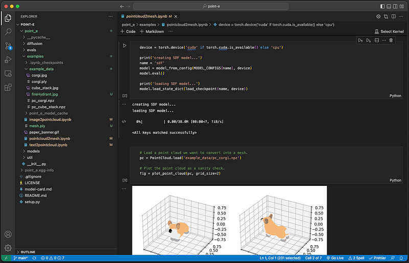
All code cells are listed, similar to Jupyter Notebook, including all execution outputs. You can make any cell active, and rerun it, just like Jupyter Notebook.

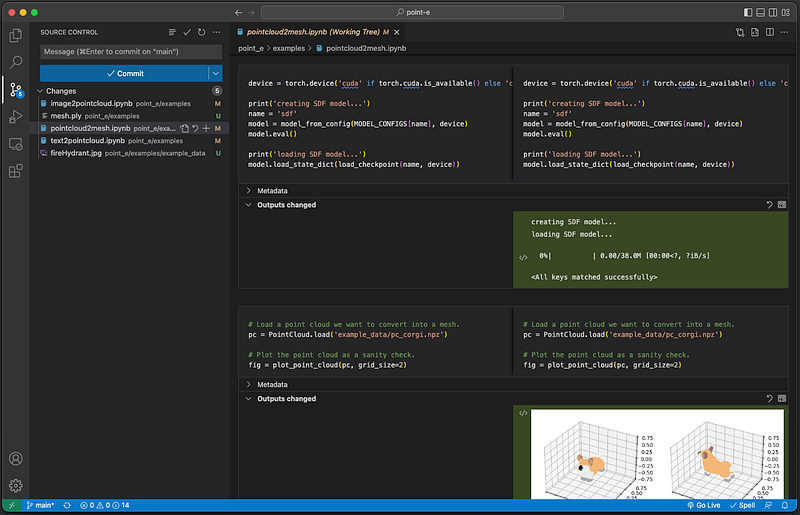
In addition, the source control view shows what have changed.

Google Colaboratory Working Environment

Lately, Google Colaboratory (Colab) becomes a popular working environment for AI computing. Colab is a free Jupyter notebook version that runs entirely in the cloud. In addition, it does not require a setup and runs with the cloud resource. It also enables collaboration among team members.

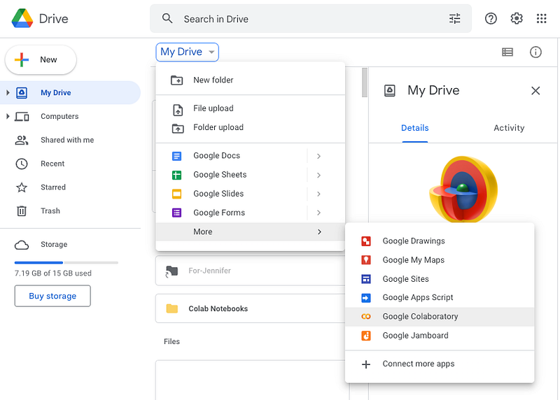
Go to https://drive.google.com/, and select My Drive → More → Google Colaboratory:

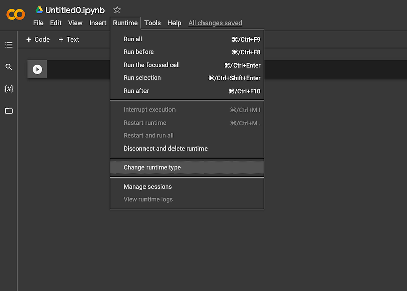
It launches an untitled notebook file. Now select Runtime → Change runtime type:

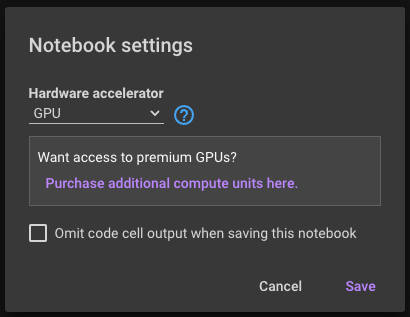
The popup modal has three choices for Hardware accelerator:

• None
• GPU: It is designed to manipulate and alter memory to accelerate the computing speed.
• TPU: It is designed to run cutting-edge machine learning models with AI services on Google Cloud.

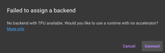
Select TPU, but it is not available.

Select GPU, and Save. Without paying for premium GPUs, the choice is only for the best effort.

At the main window, select File → Open notebook, and it pops up a modal. Go to the Github tab:

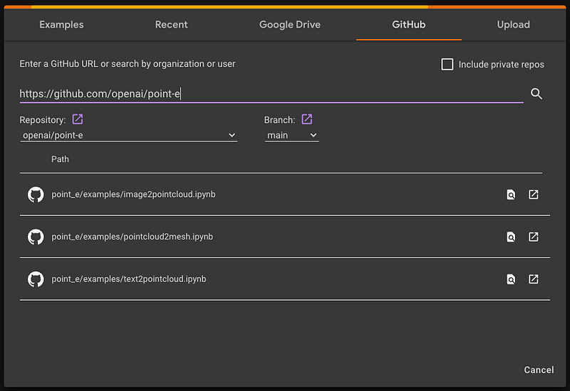
Type in the search box, https://github.com/openai/point-e, and it shows three notebook files:

• point_e/examples/image2pointcloud.ipynb
• point_e/examples/pointcloud2mesh.ipynb
• point_e/examples/text2pointcloud.ipynb

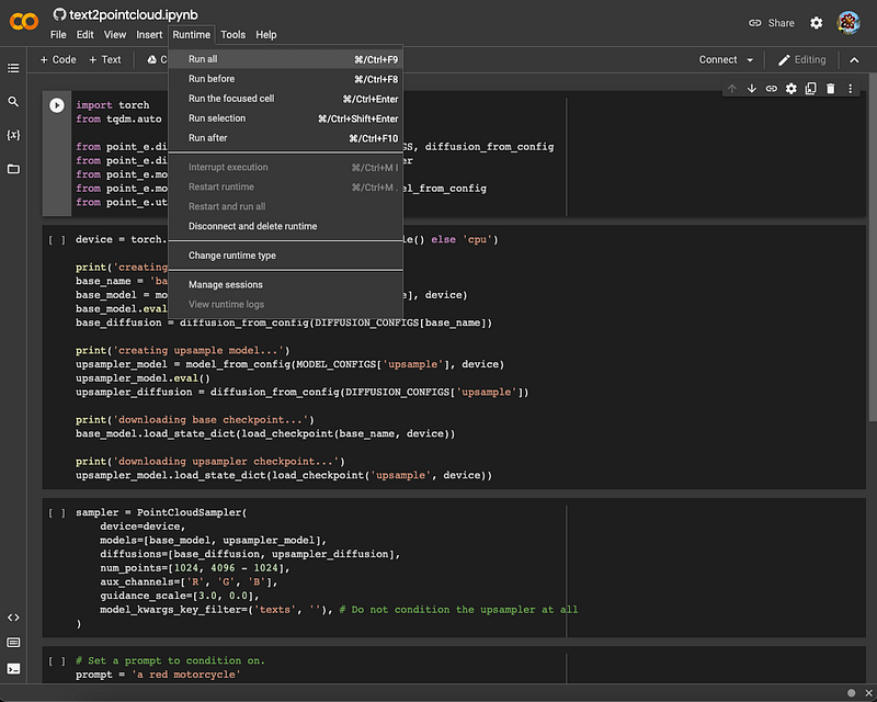
Select point_e/examples/text2pointcloud.ipynb to open it in the main window. Then, select the menu, Runtime → Run all:

The execution failed with error: ModuleNotFoundError: No module named 'point_e'.

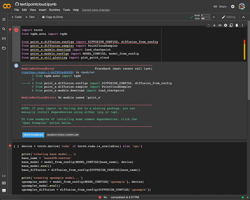
Well, text2pointcloud.ipynb cannot be executed alone. We need to clone the repository and set up the running environment.

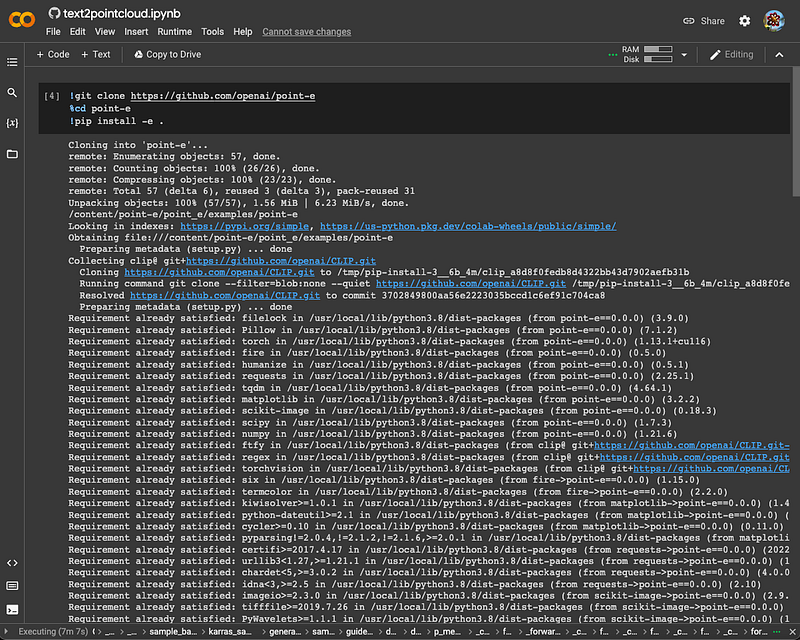
Use + Code to create a new cell at top, and add the following code in the cell:

!git clone https://github.com/openai/point-e
%cd point-e
!pip install -e .

Execute the cell:

With the running environment set, rerun text2pointcloud.ipynb.

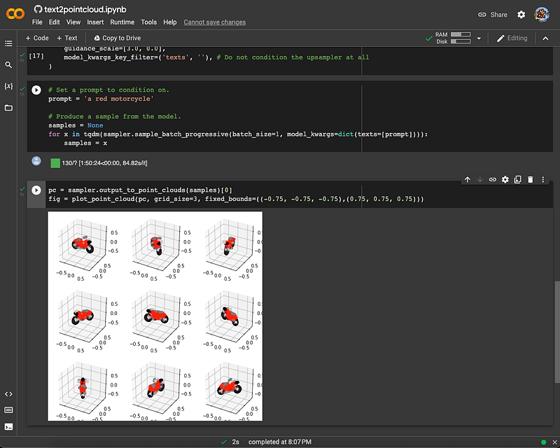
It took 1 hour 50 minutes and 24 seconds to produce a sample from the model. It is longer than running it on local, but we do not complain about using cloud resource.

At the main window, select File → Save a copy in Drive, and click the Share button. The access permission can be configured. Currently, the following link is shared by everyone.

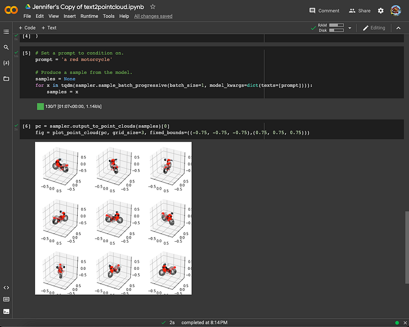
https://colab.research.google.com/drive/1VVy-YMBn7kZ5JPpPIxkyIYcb2cbHC1wq?usp=sharing

Clicking the link, and select the menu, Runtime → Run all. The program finishes in about 1 minute.

Conclusion

We have explained Point·E, a system to generate point clouds and 3D models based on descriptions and more.

On December 2022, OpenAI released the pre-trained point cloud diffusion models, as well as evaluation code and models. We have cloned the repository, and explored three examples, text-to-model, image-to-model, and 3D point cloud file to a mesh file. They work beautifully in Jupyter Notebook, Visual Studio Code, and Google Colaboratory.

Point·E is another crown jewel of OpenAI, besides DALL·E, Stable Diffusion, GPT-3, ChatGPT, and Whisper.

Thanks for reading.

Want to Connect? 

If you are interested, check out my directory of web development articles.