
Day 56: 60 days of Data Science and Machine Learning Series
ANN, Linear Regression, Decision Tree Regression and Random Forest with a project…
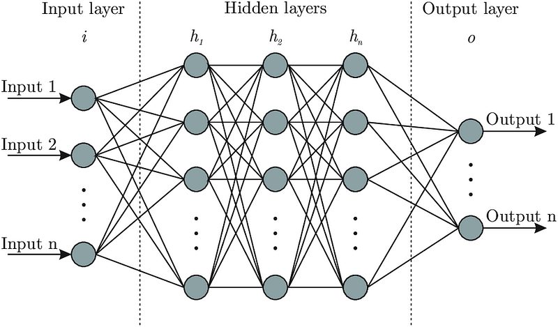
Artificial Neural Network ( ANN) is a biologically inspired computational model which consists of interconnected group of nodes and that receives inputs and gives outputs based on the predefined activation functions and internal computations.
A good reference point to understand ANN —
Some of the other best Series —
100 days : Your Data Science and Machine Learning Degree Series with projects
Complete Data Visualization and Pre-processing Series with projects
Projects Videos —
All the projects, data structures, SQL, algorithms, system design, Data Science and ML , Data Analytics, Data Engineering, , Implemented Data Science and ML projects, Implemented Data Engineering Projects, Implemented Deep Learning Projects, Implemented Machine Learning Ops Projects, Implemented Time Series Analysis and Forecasting Projects, Implemented Applied Machine Learning Projects, Implemented Tensorflow and Keras Projects, Implemented PyTorch Projects, Implemented Scikit Learn Projects, Implemented Big Data Projects, Implemented Cloud Machine Learning Projects, Implemented Neural Networks Projects, Implemented OpenCV Projects,Complete ML Research Papers Summarized, Implemented Data Analytics projects, Implemented Data Visualization Projects, Implemented Data Mining Projects, Implemented Natural Leaning Processing Projects, MLOps and Deep Learning, Applied Machine Learning with Projects Series, PyTorch with Projects Series, Tensorflow and Keras with Projects Series, Scikit Learn Series with Projects, Time Series Analysis and Forecasting with Projects Series, ML System Design Case Studies Series videos will be published on our youtube channel ( just launched).
Subscribe today!
Tech Newsletter —
If you are interested, you can join my newsletter through which I send tech interview tips, techniques, patterns, hacks — Software Development, ML, Data Science, Startups and Technology projects to more than 30K readers. You can subscribe to Tech Brew :
Simple Linear Regression
It’s a technique to estimate the relationship between two quantitative variables. It is used when you want to establish:
- Strength of the relationship — How strong the relationship is between two variables
- The value of the dependent variable at a certain value of the independent variable.
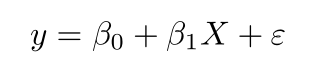
where,
y is the predicted value of the dependent variable for any given value of the independent variable which is X.
B0 is the intercept and B1 is the regression coefficient
x is the independent variable
e is the error of the estimate
Decision Tree Regression
Decision Tree are widely used in both in classification and regression problems. These are basically predictive models that use binary rules to calculate an output/target value. Each tree has branches, nodes and leaves where the root node represents the entire population or sample.
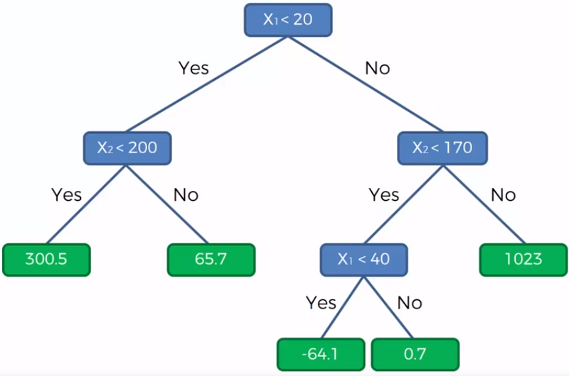
A good reference point to understand Decision Tree Regression —
Random Forest Regression
It’s a supervised machine learning algorithm that is constructed from decision tree algorithms ( it predicts the outcome by taking the average or mean of the output from the different trees) and Is used to solve both regression and classification problems. It mainly used ensemble learning, a technique in which many classifiers are combined together to provide solutions to complex problems. It’s very efficient as it reduces the overfitting of datasets, provides an effective way of handling missing data, runs efficiently on large databases, achieves extremely high accuracies, increases precision and scales really well when new features are added to the dataset..
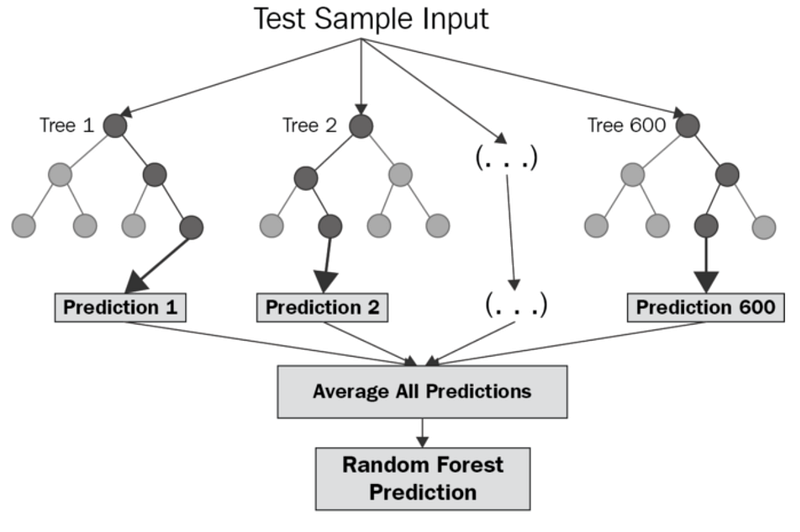
It works well with both categorical and numerical input variables, which in-turn minimizes the time spent on one-hot encoding or labeling data.
A good reference point to understand Random Forest Regression —
Let’s dive in!
Import necessary libraries
import pandas as pd
import numpy as np
import seaborn as sns
import matplotlib.pyplot as plt
import zipfile
from jupyterthemes import jtplot
jtplot.style(theme='monokai', context='notebook', ticks=True, grid=False)
from sklearn.preprocessing import StandardScaler, MinMaxScaler
from sklearn.model_selection import train_test_split
from sklearn.linear_model import LinearRegression
from sklearn.metrics import mean_squared_error, accuracy_score
from sklearn.tree import DecisionTreeRegressor
from sklearn.ensemble import RandomForestRegressor
import tensorflow as tf
from tensorflow import keras
from tensorflow.keras.layers import Dense, Activation, Dropout
from tensorflow.keras.optimizers import Adam
Load and explore data
mdf = pd.read_csv('Path ot data file/data.csv')
mdf.info()
#Check for missing values
mdf.isnull().sum()Output —
<class 'pandas.core.frame.DataFrame'>
RangeIndex: 245700 entries, 0 to 245699
Data columns (total 23 columns):
 #   Column                        Non-Null Count   Dtype
---  ------                        --------------   -----
 0   % Iron Feed                   245700 non-null  float64
 1   % Silica Feed                 245700 non-null  float64
 2   Starch Flow                   245700 non-null  float64
 3   Amina Flow                    245700 non-null  float64
 4   Ore Pulp Flow                 245700 non-null  float64
 5   Ore Pulp pH                   245700 non-null  float64
 6   Ore Pulp Density              245700 non-null  float64
 7   Flotation Column 01 Air Flow  245700 non-null  float64
 8   Flotation Column 02 Air Flow  245700 non-null  float64
 9   Flotation Column 03 Air Flow  245700 non-null  float64
 10  Flotation Column 04 Air Flow  245700 non-null  float64
 11  Flotation Column 05 Air Flow  245700 non-null  float64
 12  Flotation Column 06 Air Flow  245700 non-null  float64
 13  Flotation Column 07 Air Flow  245700 non-null  float64
 14  Flotation Column 01 Level     245700 non-null  float64
 15  Flotation Column 02 Level     245700 non-null  float64
 16  Flotation Column 03 Level     245700 non-null  float64
 17  Flotation Column 04 Level     245700 non-null  float64
 18  Flotation Column 05 Level     245700 non-null  float64
 19  Flotation Column 06 Level     245700 non-null  float64
 20  Flotation Column 07 Level     245700 non-null  float64
 21  % Iron Concentrate            245700 non-null  float64
 22  % Silica Concentrate          245700 non-null  float64
dtypes: float64(23)
memory usage: 43.1 MB
Missing values —
% Iron Feed                     0
% Silica Feed                   0
Starch Flow                     0
Amina Flow                      0
Ore Pulp Flow                   0
Ore Pulp pH                     0
Ore Pulp Density                0
Flotation Column 01 Air Flow    0
Flotation Column 02 Air Flow    0
Flotation Column 03 Air Flow    0
Flotation Column 04 Air Flow    0
Flotation Column 05 Air Flow    0
Flotation Column 06 Air Flow    0
Flotation Column 07 Air Flow    0
Flotation Column 01 Level       0
Flotation Column 02 Level       0
Flotation Column 03 Level       0
Flotation Column 04 Level       0
Flotation Column 05 Level       0
Flotation Column 06 Level       0
Flotation Column 07 Level       0
% Iron Concentrate              0
% Silica Concentrate            0
dtype: int64
Data Preprocessing
df_iron = mdf.drop(columns = '% Silica Concentrate')
df_iron_target = mdf['% Silica Concentrate']
df_iron_target = df_iron_target.reshape(-1,1)
df_iron_target.shape
#Scale
sx = StandardScaler()
X = sx.fit_transform(df_iron)sy = StandardScaler()
y = sy.fit_transform(df_iron_target)# Split the dataset
X_train, X_test, y_train, y_test = train_test_split(X,y,test_size=0.2)Linear regression model
lr_model = LinearRegression()
lr_model.fit(X_train,y_train)
alr = lr_model.score(X_test,y_test)
alr
Output —
0.6840868221951935Decision tree Regressor
dt_model = DecisionTreeRegressor()
dt_model.fit(X_train,y_train)
adt = dt_model.score(X_test,y_test)
adt
Output —
0.9835141743700436Random Forest Regressor
rf_model = RandomForestRegressor(n_estimators=100,max_depth = 10)
rf_model.fit(X_train,y_train)
arf = rf_model.score(X_test,y_test)
arfOutput —
0.8944514292225525Artificial Neural Network
optimizer = Adam(learning_rate=0.001, beta_1 = 0.9, beta_2 = 0.999, epsilon = 1e-07, amsgrad = False)
ANN_model = keras.Sequential()
ANN_model.add(Dense(250, input_dim = 22, kernel_initializer='normal',activation='relu'))
ANN_model.add(Dense(500,activation = 'relu'))
ANN_model.add(Dropout(0.1))
ANN_model.add(Dense(1000, activation = 'relu'))
ANN_model.add(Dropout(0.1))
ANN_model.add(Dense(1000, activation = 'relu'))
ANN_model.add(Dropout(0.1))
ANN_model.add(Dense(500, activation = 'relu'))
ANN_model.add(Dropout(0.1))
ANN_model.add(Dense(250, activation = 'relu'))
ANN_model.add(Dropout(0.1))
ANN_model.add(Dense(250, activation = 'relu'))
ANN_model.add(Dropout(0.1))
ANN_model.add(Dense(1, activation = 'linear'))
ANN_model.compile(loss = 'mse', optimizer = 'adam')
ANN_model.summary()
Output —
Model: "sequential"
_________________________________________________________________
Layer (type)                 Output Shape              Param #
=================================================================
dense (Dense)                (None, 250)               5750
_________________________________________________________________
dense_1 (Dense)              (None, 500)               125500
_________________________________________________________________
dropout (Dropout)            (None, 500)               0
_________________________________________________________________
dense_2 (Dense)              (None, 1000)              501000
_________________________________________________________________
dropout_1 (Dropout)          (None, 1000)              0
_________________________________________________________________
dense_3 (Dense)              (None, 1000)              1001000
_________________________________________________________________
dropout_2 (Dropout)          (None, 1000)              0
_________________________________________________________________
dense_4 (Dense)              (None, 500)               500500
_________________________________________________________________
dropout_3 (Dropout)          (None, 500)               0
_________________________________________________________________
dense_5 (Dense)              (None, 250)               125250
_________________________________________________________________
dropout_4 (Dropout)          (None, 250)               0
_________________________________________________________________
dense_6 (Dense)              (None, 250)               62750
_________________________________________________________________
dropout_5 (Dropout)          (None, 250)               0
_________________________________________________________________
dense_7 (Dense)              (None, 1)                 251
=================================================================
Total params: 2,322,001
Trainable params: 2,322,001
Non-trainable params: 0
history = ANN_model.fit(X_train,y_train, epochs = 5, validation_split = 0.2)
result = ANN_model.evaluate(X_test, y_test)
accuracy_ANN = 1 - result
plt.plot(history.history['loss'])
plt.plot(history.history['val_loss'])
plt.title('Model loss')
plt.ylabel('loss')
plt.xlabel('epoch')
plt.legend(['train_loss','val_loss'], loc = 'upper right')
plt.show()Output —
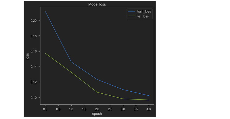
Learnings —
How to train ANN and perform regression task and understand/implement Regression model KPI’s.
Day 57: Coming soon!
Follow and Stay tuned. Keep coding :)
For other projects, tune to —
Build Machine Learning Pipelines( With Code)
Recurrent Neural Network with Keras
Clustering Geolocation Data in Python using DBSCAN and K-Means
Facial Expression Recognition using Keras
Hyperparameter Tuning with Keras Tuner
Custom Layers in Keras
That’s it fellas. Peace out and keep coding :)
Stay Tuned and of-course let me end this post with a quote by Steve Jobs ;)
“You have to be burning with an idea, or a problem, or a wrong that you want to right. If you’re not passionate enough from the start, you’ll never stick it out.”


