
Day 38: 60 days of Data Science and Machine Learning Series
Support Vector Machine with a project..
Welcome back peeps. In this post we are going to implement Support Vector Machine with a project.
Some of the other best Series —
100 days : Your Data Science and Machine Learning Degree Series with projects
Complete Data Visualization and Pre-processing Series with projects
Projects Videos —
All the projects, data structures, SQL, algorithms, system design, Data Science and ML , Data Analytics, Data Engineering, , Implemented Data Science and ML projects, Implemented Data Engineering Projects, Implemented Deep Learning Projects, Implemented Machine Learning Ops Projects, Implemented Time Series Analysis and Forecasting Projects, Implemented Applied Machine Learning Projects, Implemented Tensorflow and Keras Projects, Implemented PyTorch Projects, Implemented Scikit Learn Projects, Implemented Big Data Projects, Implemented Cloud Machine Learning Projects, Implemented Neural Networks Projects, Implemented OpenCV Projects,Complete ML Research Papers Summarized, Implemented Data Analytics projects, Implemented Data Visualization Projects, Implemented Data Mining Projects, Implemented Natural Leaning Processing Projects, MLOps and Deep Learning, Applied Machine Learning with Projects Series, PyTorch with Projects Series, Tensorflow and Keras with Projects Series, Scikit Learn Series with Projects, Time Series Analysis and Forecasting with Projects Series, ML System Design Case Studies Series videos will be published on our youtube channel ( just launched).
Subscribe today!
Tech Newsletter —
If you are interested, you can join my newsletter through which I send tech interview tips, techniques, patterns, hacks — Software Development, ML, Data Science, Startups and Technology projects to more than 30K readers. You can subscribe to Tech Brew :
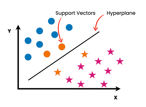
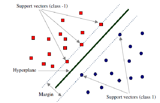
Support Vector Machine is a supervised machine learning algorithm which is used for both classification or regression problems. In this technique we start by plotting each data item as point in n-dimensional space with the value of a particular coordinate as being the value of the feature/independent variable. Then, we find the hyper-plane that differentiates the two classes by a boundary as shown in the image below.
The data for this project can be found at
Let’s dive in!
Importing necessary libraries
import numpy as np
import matplotlib.pyplot as plt
import pandas as pd
from sklearn.model_selection import train_test_split
from sklearn.preprocessing import StandardScaler
from sklearn.svm import SVC
from sklearn.metrics import confusion_matrix
from matplotlib.colors import ListedColormap
Load the dataset
# Importing the dataset
dataset = pd.read_csv('/Path to file/datav1.2.csv')
X = dataset.iloc[:, [2, 3]].values
Y = dataset.iloc[:, 4].values
Split the dataset
X_train, X_test, Y_train, Y_test = train_test_split(X, Y, test_size = 0.25, random_state = 0)Feature Scaling for normalization
sc = StandardScaler()
X_train = sc.fit_transform(X_train)
X_test = sc.transform(X_test)
Model Fitting and Predictions
svmclassifier = SVC(kernel = 'linear' , random_state = 0)
svmclassifier.fit (X_train, Y_train)
Y_pred = svmclassifier.predict(X_test)
Confusion Matrix
cm = confusion_matrix(Y_test, Y_pred)Visualize the training set results
X_set, Y_set = X_train, Y_train
X1, X2 = np.meshgrid(np.arange(start = X_set[:, 0].min() - 1, stop = X_set[:, 0].max() + 1, step = 0.01),
np.arange(start = X_set[:, 1].min() - 1, stop = X_set[:, 1].max() + 1, step = 0.01))
plt.contourf(X1, X2, svmclassifier.predict(np.array([X1.ravel(), X2.ravel()]).T).reshape(X1.shape),
alpha = 0.75, cmap = ListedColormap(('red', 'blue')))
plt.xlim(X1.min(), X1.max())
plt.ylim(X2.min(), X2.max())
for i, j in enumerate(np.unique(Y_set)):
plt.scatter(X_set[Y_set == j, 0], X_set[Y_set == j, 1],
c = ListedColormap(('red', 'blue'))(i), label = j)
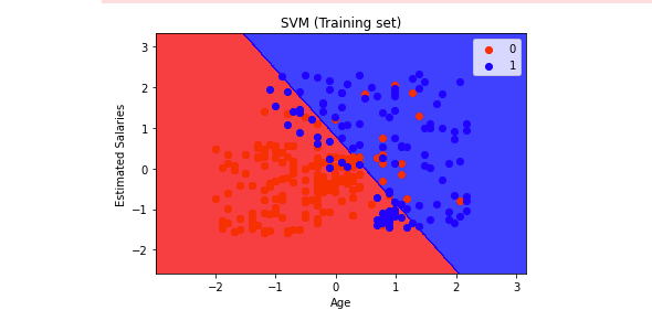
plt.title('SVM (Training set)')
plt.xlabel('Age')
plt.ylabel('Estimated Salaries')
plt.legend()
plt.show()Output —
Visualize the testing set results
X_set, Y_set = X_test, Y_test
X1, X2 = np.meshgrid(np.arange(start = X_set[:, 0].min() - 1, stop = X_set[:, 0].max() + 1, step = 0.01),
np.arange(start = X_set[:, 1].min() - 1, stop = X_set[:, 1].max() + 1, step = 0.01))
plt.contourf(X1, X2, svmclassifier.predict(np.array([X1.ravel(), X2.ravel()]).T).reshape(X1.shape),
alpha = 0.75, cmap = ListedColormap(('red', 'blue')))
plt.xlim(X1.min(), X1.max())
plt.ylim(X2.min(), X2.max())
for i, j in enumerate(np.unique(Y_set)):
plt.scatter(X_set[Y_set == j, 0], X_set[Y_set == j, 1],
c = ListedColormap(('red', 'blue'))(i), label = j)
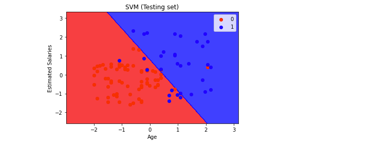
plt.title('SVM (Testing set)')
plt.xlabel('Age')
plt.ylabel('Estimated Salaries')
plt.legend()
plt.show()Output —
Day 39 : Coming soon!
Follow and Stay tuned. Keep coding :)
For other projects, tune to —
Build Machine Learning Pipelines( With Code)
Recurrent Neural Network with Keras
Clustering Geolocation Data in Python using DBSCAN and K-Means
Facial Expression Recognition using Keras
Hyperparameter Tuning with Keras Tuner
Custom Layers in Keras
That’s it fellas. Peace out and keep coding :)
Stay Tuned and of-course let me end this post with a quote by Steve Jobs ;)
“You have to be burning with an idea, or a problem, or a wrong that you want to right. If you’re not passionate enough from the start, you’ll never stick it out.”


