Day 35: 60 days of Data Science and Machine Learning Series

Principal Component Analysis with a project..

Dimensionality is the number of input variables or features for a dataset and dimensionality reduction is the process through which we reduce the number of input variables in a dataset. A lot of input features makes predictive modeling a more challenging task.

Some of the other best Series —

30 Days of Natural Language Processing ( NLP) Series

30 days of Data Engineering with projects Series

60 days of Data Science and ML Series with projects

100 days : Your Data Science and Machine Learning Degree Series with projects

23 Data Science Techniques You Should Know

Tech Interview Series — Curated List of coding questions

Complete System Design with most popular Questions Series

Complete Data Visualization and Pre-processing Series with projects

Complete Python Series with Projects

Complete Advanced Python Series with Projects

Kaggle Best Notebooks that will teach you the most

Complete Developers Guide to Git

All the Data Science and Machine Learning Resources

210 Machine Learning Projects

30 days of Machine Learning Ops

Projects Videos —

All the projects, data structures, SQL, algorithms, system design, Data Science and ML , Data Analytics, Data Engineering, , Implemented Data Science and ML projects, Implemented Data Engineering Projects, Implemented Deep Learning Projects, Implemented Machine Learning Ops Projects, Implemented Time Series Analysis and Forecasting Projects, Implemented Applied Machine Learning Projects, Implemented Tensorflow and Keras Projects, Implemented PyTorch Projects, Implemented Scikit Learn Projects, Implemented Big Data Projects, Implemented Cloud Machine Learning Projects, Implemented Neural Networks Projects, Implemented OpenCV Projects,Complete ML Research Papers Summarized, Implemented Data Analytics projects, Implemented Data Visualization Projects, Implemented Data Mining Projects, Implemented Natural Leaning Processing Projects, MLOps and Deep Learning, Applied Machine Learning with Projects Series, PyTorch with Projects Series, Tensorflow and Keras with Projects Series, Scikit Learn Series with Projects, Time Series Analysis and Forecasting with Projects Series, ML System Design Case Studies Series videos will be published on our youtube channel ( just launched).

Subscribe today!

Tech Newsletter —

If you are interested, you can join my newsletter through which I send tech interview tips, techniques, patterns, hacks — Software Development, ML, Data Science, Startups and Technology projects to more than 30K readers. You can subscribe to Tech Brew :

Principal Component Analysis is a dimensionality-reduction technique used to reduce the dimensionality of large data sets to smaller one, by transforming a large set of variables while preserving the information all along.

In this post, we are going to demonstrate PCA. Data for this project can be found here:

https://archive.ics.uci.edu/ml/machine-learning-databases/iris/iris.data

Let’s dive in!

Import necessary libraries

%matplotlib inline
import pandas as pd
import matplotlib.pyplot as plt
import numpy as np
import seaborn as sns
from sklearn.preprocessing import StandardScaler
plt.style.use("ggplot")
plt.rcParams["figure.figsize"] = (15,10)

Load the Data

iris = pd.read_csv('Path to data",header= None)
iris.info()

Output —

<class 'pandas.core.frame.DataFrame'>
Int64Index: 150 entries, 0 to 149
Data columns (total 5 columns):
sepal_length    150 non-null float64
sepal_width     150 non-null float64
petal_length    150 non-null float64
petal_width     150 non-null float64
species         150 non-null object
dtypes: float64(4), object(1)
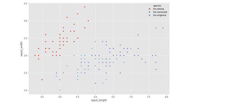
memory usage: 7.0+ KB

Data Visualization

sns.scatterplot(x=iris.sepal_length,y=iris.sepal_width,hue=iris.species,style=iris.species)

Output —

Data Standardization

X = iris.iloc[:,0:4].values
y=iris.species.values

X= StandardScaler().fit_transform(X)

Compute the Eigenvectors and Eigenvalues

covariance_matrix = np.cov(X.T)
eigen_values, eigen_vectors = np.linalg.eig(covariance_matrix)
print("Eigen Values:",eigen_values)

print("Eigen Vectors:", eigen_vectors)

Output —

Eigen Values: [2.93035378 0.92740362 0.14834223 0.02074601]
Eigen Vectors: [[ 0.52237162 -0.37231836 -0.72101681  0.26199559]
 [-0.26335492 -0.92555649  0.24203288 -0.12413481]
 [ 0.58125401 -0.02109478  0.14089226 -0.80115427]
 [ 0.56561105 -0.06541577  0.6338014   0.52354627]]

Singular Value Decomposition (SVD)

eigen_svd, s, v = np.linalg.svd(X.T)
eigen_svd

Output —

array([[-0.52237162, -0.37231836,  0.72101681,  0.26199559],
       [ 0.26335492, -0.92555649, -0.24203288, -0.12413481],
       [-0.58125401, -0.02109478, -0.14089226, -0.80115427],
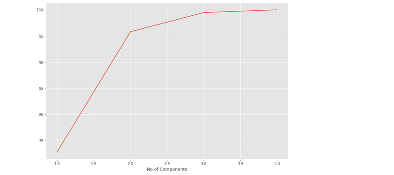
       [-0.56561105, -0.06541577, -0.6338014 ,  0.52354627]])

Principal Components

var_e = [(i/sum(eigen_values))*100 for i in eigen_values]
sns.lineplot(x=[1,2,3,4],y=np.cumsum(var_e))
plt.xlabel("No of Components")
plt.show()

Output —

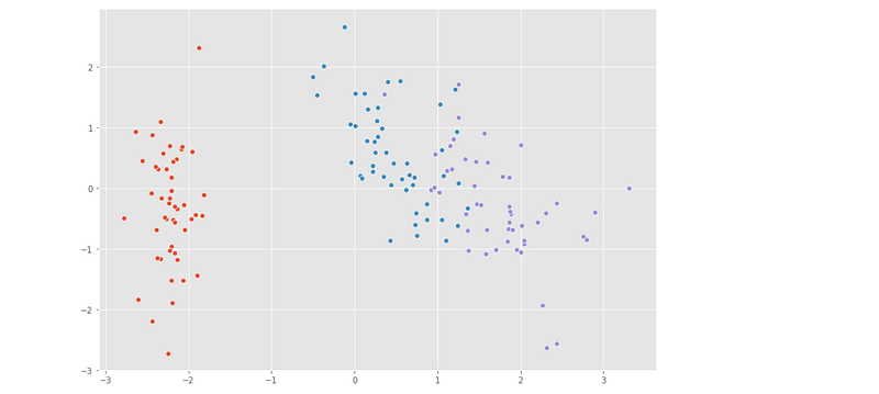
Plot Data

p_m = (eigen_vectors.T[:][:])[:2].T
X_pca = X.dot(p_m)

for species in ('Iris-setosa','Iris-versicolor','Iris-virginica'):
    sns.scatterplot(X_pca[y==species,0],
                   X_pca[y==species,1])

Output —

Day 36 : Coming soon

Follow and Stay tuned. Keep coding :)

For other projects, tune to —

Build Machine Learning Pipelines( With Code)

Recurrent Neural Network with Keras

Clustering Geolocation Data in Python using DBSCAN and K-Means

Facial Expression Recognition using Keras

Hyperparameter Tuning with Keras Tuner

Custom Layers in Keras

That’s it fellas. Peace out and keep coding :)

Stay Tuned and of-course let me end this post with a quote by Steve Jobs ;)

“You have to be burning with an idea, or a problem, or a wrong that you want to right. If you’re not passionate enough from the start, you’ll never stick it out.”