
Day 34: 60 days of Data Science and Machine Learning Series
Regression Project 4..
Welcome back peeps. In this post we will cover logistic regression with a project.
Some of the other best Series —
100 days : Your Data Science and Machine Learning Degree Series with projects
Complete Data Visualization and Pre-processing Series with projects
Projects Videos —
All the projects, data structures, SQL, algorithms, system design, Data Science and ML , Data Analytics, Data Engineering, , Implemented Data Science and ML projects, Implemented Data Engineering Projects, Implemented Deep Learning Projects, Implemented Machine Learning Ops Projects, Implemented Time Series Analysis and Forecasting Projects, Implemented Applied Machine Learning Projects, Implemented Tensorflow and Keras Projects, Implemented PyTorch Projects, Implemented Scikit Learn Projects, Implemented Big Data Projects, Implemented Cloud Machine Learning Projects, Implemented Neural Networks Projects, Implemented OpenCV Projects,Complete ML Research Papers Summarized, Implemented Data Analytics projects, Implemented Data Visualization Projects, Implemented Data Mining Projects, Implemented Natural Leaning Processing Projects, MLOps and Deep Learning, Applied Machine Learning with Projects Series, PyTorch with Projects Series, Tensorflow and Keras with Projects Series, Scikit Learn Series with Projects, Time Series Analysis and Forecasting with Projects Series, ML System Design Case Studies Series videos will be published on our youtube channel ( just launched).
Subscribe today!
Tech Newsletter —
If you are interested, you can join my newsletter through which I send tech interview tips, techniques, patterns, hacks — Software Development, ML, Data Science, Startups and Technology projects to more than 30K readers. You can subscribe to Tech Brew :
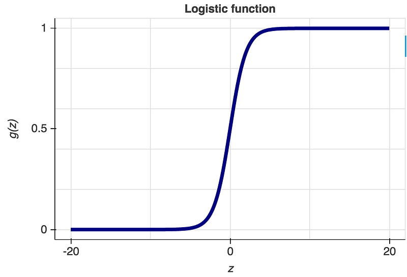
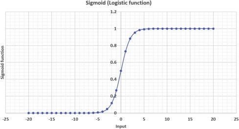
In logistic regression, we establish the relationship between the dependent variable and one or more independent variables by estimating probabilities using an equation ( logistic regression).
Let’s dive in!
Import necessary libraries
import random
import numpy as np
import warnings
import helpers.plt, helpers.dataset
from matplotlib import pyplot as plt
%matplotlib inline
warnings.filterwarnings('ignore')
Set Hyperparameters
These are the parameters ( examples as listed below) that is set before the learning process begins, are tunable and can directly affect how well a model trains.
- Learning Rate
- Regularization constant
- Number of branches, Number of epochs
- Number of clusters etc
lr = 0.3
batch_size = 300
iterations = 40
Load the Dataset
(X_train,Y_train), (X_test,Y_test) = helpers.dataset.get_data()
print('Shape of X_train:', X_train.shape)
print('Shape of Y_train:', Y_train.shape)
print('Shape of X_test:', X_test.shape)
print('Shape of Y_test:', Y_test.shape)
Output —
Shape of X_train: (12665, 28, 28)
Shape of Y_train: (12665,)
Shape of X_test: (2115, 28, 28)
Shape of Y_test: (2115,)
Create Model
A logistic model is simply a multi variable linear equation which gives a binary output.
class LogisticModel:
    def __init__(self, num_features):

        self.W = np.reshape(np.random.randn((num_features)),
                 (num_features,1))
        self.b = np.zeros((1,1))
        self.num_features = num_features
        self.losses = []
        self.accuracies =[]
    def summary(self):

        print('Number of features:', self.num_features)
        print('Shape of weights:', self.W.shape)
        print('Shape of biases:', self.b.shape)


model = LogisticModel(num_features=784)
model.summary()
Output —
Number of features: 784
Shape of weights: (784, 1)
Shape of biases: (1, 1)
Forward Pass
class LogisticModel(LogisticModel):
    def _forward_pass(self, X, Y=None):

        batch_size = X.shape[0]
        Z = np.dot(X,self.W) +self.b
        A = 1./(1. +np.exp(-Z))
        loss = float(1e6)
        if Y is not None:
            loss = -1 * np.sum(np.dot(np.transpose(Y),\
            np.log(A))+  np.matmul(np.transpose(1-Y),np.log(1-A)))
            loss /= batch_size
        return A,loss
Backward Pass
class LogisticModel(LogisticModel):
    def _backward_pass(self, A, X, Y):

        batch_size = X.shape[0]
        dZ=A-Y
        dW = np.dot(np.transpose(X),dZ) / batch_size
        db = np.sum(dZ) /batch_size
        return dW,db
Update Parameters
class LogisticModel(LogisticModel):
    def _update_params(self, dW, db, lr):

        self.W -= lr * dW
        self.b -= lr * db
Check Model Performance
class LogisticModel(LogisticModel):
    def predict(self, X, Y=None):

        A,loss = self._forward_pass(X,Y)
        Y_hat = A > 0.5
        return np.squeeze(Y_hat),loss

    def evaluate(self, X, Y):

        Y_hat,loss = self.predict(X,Y)
        accuracy = np.sum(Y_hat == np.squeeze(Y))/ X.shape[0]
        return accuracy, loss
model =LogisticModel(784)
model.summary()X,Y = helpers.dataset.get_random_batch(X_test,Y_test,batch_size)
acc,loss = model.evaluate(X,Y)
print("Accuracy:", acc)
print("Loss:", loss)Output —
Number of features: 784
Shape of weights: (784, 1)
Shape of biases: (1, 1)

Accuracy: 0.25
Loss : 5.139016761351013
Training Loop
class LogisticModel(LogisticModel):
    def train(self, batch_size, get_batch, lr, iterations, X_train,
              Y_train, X_test, Y_test):

        self.accuracies = []
        self.losses = []

        for i in range(iterations):
            X,Y = get_batch(X_train,Y_train,batch_size)
            A,_ = self._forward_pass(X,Y)
            dW,db = self._backward_pass(A,X,Y)
            self._update_params(dW,db,lr)

            X,Y = get_batch(X_test,Y_test,batch_size)
            val_acc,val_loss = self.evaluate(X,Y)
            self.accuracies.append(val_acc)
            self.losses.append(val_loss)
            print(i,val_acc,val_loss)
Model Training and Results
model = LogisticModel(784)X,Y = helpers.dataset.get_random_batch(X_test,Y_test,batch_size)model.train(
batch_size,
helpers.dataset.get_random_batch,
lr, iterations, X_train, Y_train,
X_test,Y_test)
print(model.evaluate(X,Y))Output —
0 0.38333333333333336 2.9112418287841
1 0.58 1.0920400376536754
2 0.8033333333333333 0.4733993185165991
3 0.8566666666666667 0.3860987796373691
4 0.92 0.22385032248466283
5 0.9433333333333334 0.16269221395977546
6 0.9533333333333334 0.13423627297149432
7 0.9333333333333333 0.1867625304499955
8 0.9766666666666667 0.08768901259572759
9 0.9733333333333334 0.09854519582688483
10 0.9766666666666667 0.07597673045261207
11 0.9766666666666667 0.0906360847939501
12 0.97 0.09736912192570973
13 0.99 0.05219127708236699
14 0.9833333333333333 0.06803636200857319
15 0.9766666666666667 0.05909810278419808
16 0.9733333333333334 0.04908840771386662
17 0.9666666666666667 0.11160536628554771
18 0.99 0.04569546767029207
19 0.9833333333333333 0.0630524474725281
20 0.9866666666666667 0.027689980368903376
21 0.9866666666666667 0.04844713667127785
22 0.99 0.03169328394070209
23 0.99 0.04417471252597749
24 0.99 0.03170499943380271
25 0.9933333333333333 0.012347557895914048
26 0.9833333333333333 0.05861541302888874
27 0.99 0.02411309909197451
28 0.9766666666666667 0.03870235621447865
29 0.9933333333333333 0.01807624105597577
30 0.9933333333333333 0.014707446692389648
31 0.9733333333333334 0.1001476449251274
32 0.9833333333333333 0.06153675229309561
33 0.9866666666666667 0.025670351820764055
34 0.9933333333333333 0.015290944469583451
35 0.99 0.023528542612788743
36 0.9933333333333333 0.01986740723553504
37 0.99 0.018890984240146534
38 0.98 0.050996656197463665
39 0.9966666666666667 0.01599068224616575
(0.9933333333333333, 0.026105419192584314)
Plot the results
helpers.plt.plot_metrics(model)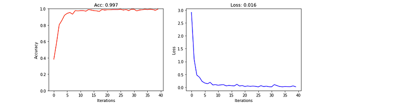
Day 35 : Coming soon
Follow and Stay tuned. Keep coding :)
For other projects, tune to —
Build Machine Learning Pipelines( With Code)
Recurrent Neural Network with Keras
Clustering Geolocation Data in Python using DBSCAN and K-Means
Facial Expression Recognition using Keras
Hyperparameter Tuning with Keras Tuner
Custom Layers in Keras
That’s it fellas. Peace out and keep coding :)
Stay Tuned and of-course let me end this post with a quote by Steve Jobs ;)
“You have to be burning with an idea, or a problem, or a wrong that you want to right. If you’re not passionate enough from the start, you’ll never stick it out.”


