
Day 33: 60 days of Data Science and Machine Learning Series
Regression Project 3..
Welcome back peeps. In this post we will cover logistic regression with a project.
Simple Linear Regression
It’s a technique to estimate the relationship between two quantitative variables. It is used when you want to establish:
- Strength of the relationship — How strong the relationship is between two variables
- The value of the dependent variable at a certain value of the independent variable.
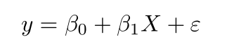
where,
y is the predicted value of the dependent variable for any given value of the independent variable which is X.
B0 is the intercept and B1 is the regression coefficient
x is the independent variable
e is the error of the estimate
Some of the other best Series —
100 days : Your Data Science and Machine Learning Degree Series with projects
Complete Data Visualization and Pre-processing Series with projects
Projects Videos —
All the projects, data structures, SQL, algorithms, system design, Data Science and ML , Data Analytics, Data Engineering, , Implemented Data Science and ML projects, Implemented Data Engineering Projects, Implemented Deep Learning Projects, Implemented Machine Learning Ops Projects, Implemented Time Series Analysis and Forecasting Projects, Implemented Applied Machine Learning Projects, Implemented Tensorflow and Keras Projects, Implemented PyTorch Projects, Implemented Scikit Learn Projects, Implemented Big Data Projects, Implemented Cloud Machine Learning Projects, Implemented Neural Networks Projects, Implemented OpenCV Projects,Complete ML Research Papers Summarized, Implemented Data Analytics projects, Implemented Data Visualization Projects, Implemented Data Mining Projects, Implemented Natural Leaning Processing Projects, MLOps and Deep Learning, Applied Machine Learning with Projects Series, PyTorch with Projects Series, Tensorflow and Keras with Projects Series, Scikit Learn Series with Projects, Time Series Analysis and Forecasting with Projects Series, ML System Design Case Studies Series videos will be published on our youtube channel ( just launched).
Subscribe today!
Tech Newsletter —
If you are interested, you can join my newsletter through which I send tech interview tips, techniques, patterns, hacks — Software Development, ML, Data Science, Startups and Technology projects to more than 30K readers. You can subscribe to Tech Brew :
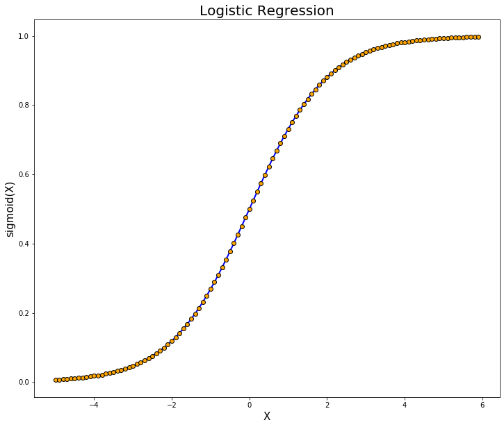
In logistic regression, we establish the relationship between the dependent variable and one or more independent variables by estimating probabilities using an equation ( logistic regression).
Data for this project can be accessed here :
Let’s dive in!
Import necessary libraries
import numpy as np
import matplotlib.pyplot as plt
import seaborn as sns
import pandas as pd
plt.style.use("ggplot")
%matplotlib inline
from pylab import rcParams
rcParams['figure.figsize'] = 15, 10
Load the Data
dt = pd.read_csv('Path to the file')
dt.info()
Output —
<class 'pandas.core.frame.DataFrame'>
RangeIndex: 100 entries, 0 to 99
Data columns (total 3 columns):
DMV_Test_1    100 non-null float64
DMV_Test_2    100 non-null float64
Results       100 non-null int64
dtypes: float64(2), int64(1)
memory usage: 2.4 KB
Data Visualization
scores = dt[['DMV_Test_1','DMV_Test_2']].values
results = dt['Results'].values
p = (results==1).reshape(100,1)
f = (results==0).reshape(100,1)ax=sns.scatterplot(x=scores[p[:,0],0],
y=scores[p[:,0],1],
marker="^",
color='green',
s=60)
sns.scatterplot(x=scores[f[:,0],0],
y=scores[f[:,0],1],
marker="o",
color='blue',
s=60)
ax.set(xlabel='Test 1 Scores',ylabel='Test 2 scores')
ax.legend(['Passed','Failed'])
plt.show();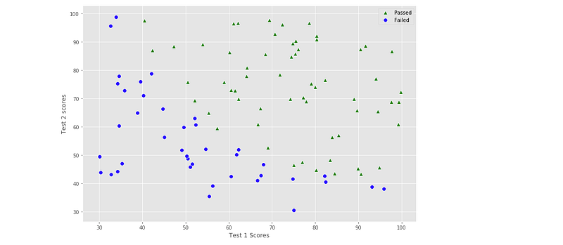
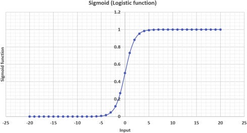
Define the Logistic Sigmoid Function 𝜎(𝑧)
def logistic_function(x):
    return 1/(1+np.exp(-x))
logistic_function(0)
Output —
0.5Compute the Cost Function 𝐽(𝜃) and Gradient
def compute_cost(theta,x,y):
    m=len(y)
    y_pred =logistic_function(np.dot(x,theta))
    error = (y * np.log(y_pred)) +(1-y) * np.log(1-y_pred)
    cost = -1/m * sum(error)
    gradient = 1/m * np.dot(x.transpose(),(y_pred - y))
    return cost[0],gradient
Cost and Gradient
mean_scores = np.mean(scores,axis=0)
std_scores = np.std(scores, axis=0)
scores = ( scores - mean_scores)/std_scores
rows = scores.shape[0]
cols = scores.shape[1]X=np.append(np.ones((rows,1)),scores,axis=1)
y=results.reshape(rows,1)theta_init = np.zeros((cols+1,1))
cost,gradient = compute_cost(theta_init,X,y)print('Cost : ',cost)
print('Gradient : ',gradient)Output —
Cost 0.693147180559946
Gradient
[[-0.1       ]
 [-0.28122914]
 [-0.25098615]]
Implement Gradient Descent
def gradient_descent(x,y,theta,alpha,iterations):
    costs = []
    for i in range(iterations):
        cost,gradient = compute_cost(theta,x,y)
        theta -= (alpha * gradient)
        costs.append(cost)
    return theta,costs
theta, costs = gradient_descent(X,y,theta_init,1,200)
print('Theta: ',theta)
print('Resulting Cost: ',costs[-1])
Output —
Theta
[[1.50850586]
 [3.5468762 ]
 [3.29383709]]
Resulting Cost 0.2048938203512014
Plotting the Convergence of 𝐽(𝜃)
plt.plot(costs)
plt.xlabel('Iterations')
plt.ylabel('$J(\Theta)$')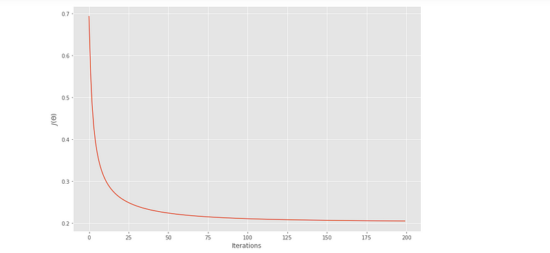
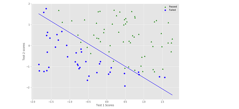
Plotting the Decision Boundary
ax=sns.scatterplot(x=X[p[:,0],1],
                  y=X[p[:,0],2],
                  marker="^",
                  color='green',
                  s=60)
sns.scatterplot(x=X[f[:,0],1],
                  y=X[f[:,0],2],
                  marker="o",
                  color='blue',
                  s=60)
ax.set(xlabel='Test 1 Scores',ylabel='Test 2 scores')
ax.legend(['Passed','Failed'])
x_boundary = np.array([np.min(X[:,1]),np.max([X[:,1]])])
y_boundary = -(theta[0] + theta[1] * x_boundary)/theta[2]sns.lineplot(x=x_boundary,y=y_boundary,color='blue')plt.show();Output —
ML Regression Project 4: Coming soon
Follow and Stay tuned. Keep coding :)
For other projects, tune to —
Build Machine Learning Pipelines( With Code)
Recurrent Neural Network with Keras
Clustering Geolocation Data in Python using DBSCAN and K-Means
Facial Expression Recognition using Keras
Hyperparameter Tuning with Keras Tuner
Custom Layers in Keras
That’s it fellas. Peace out and keep coding :)
Stay Tuned and of-course let me end this post with a quote by Steve Jobs ;)
“Remembering that you are going to die is the best way I know to avoid the trap of thinking you have something to lose. You are already naked. There is no reason not to follow your heart.”


