
Day 31: 60 days of Data Science and Machine Learning Series
Regression Project 1..
Welcome back peeps. Finally, holidays have started and work has taken a back seat. I have ample time now so, I intend to complete this series in the last 12 days of 2021.
Some of the other best Series —
100 days : Your Data Science and Machine Learning Degree Series with projects
Complete Data Visualization and Pre-processing Series with projects
Projects Videos —
All the projects, data structures, SQL, algorithms, system design, Data Science and ML , Data Analytics, Data Engineering, , Implemented Data Science and ML projects, Implemented Data Engineering Projects, Implemented Deep Learning Projects, Implemented Machine Learning Ops Projects, Implemented Time Series Analysis and Forecasting Projects, Implemented Applied Machine Learning Projects, Implemented Tensorflow and Keras Projects, Implemented PyTorch Projects, Implemented Scikit Learn Projects, Implemented Big Data Projects, Implemented Cloud Machine Learning Projects, Implemented Neural Networks Projects, Implemented OpenCV Projects,Complete ML Research Papers Summarized, Implemented Data Analytics projects, Implemented Data Visualization Projects, Implemented Data Mining Projects, Implemented Natural Leaning Processing Projects, MLOps and Deep Learning, Applied Machine Learning with Projects Series, PyTorch with Projects Series, Tensorflow and Keras with Projects Series, Scikit Learn Series with Projects, Time Series Analysis and Forecasting with Projects Series, ML System Design Case Studies Series videos will be published on our youtube channel ( just launched).
Subscribe today!
Tech Newsletter —
If you are interested, you can join my newsletter through which I send tech interview tips, techniques, patterns, hacks — Software Development, ML, Data Science, Startups and Technology projects to more than 30K readers. You can subscribe to Tech Brew :
In this post we will cover univariate linear regression with a project.
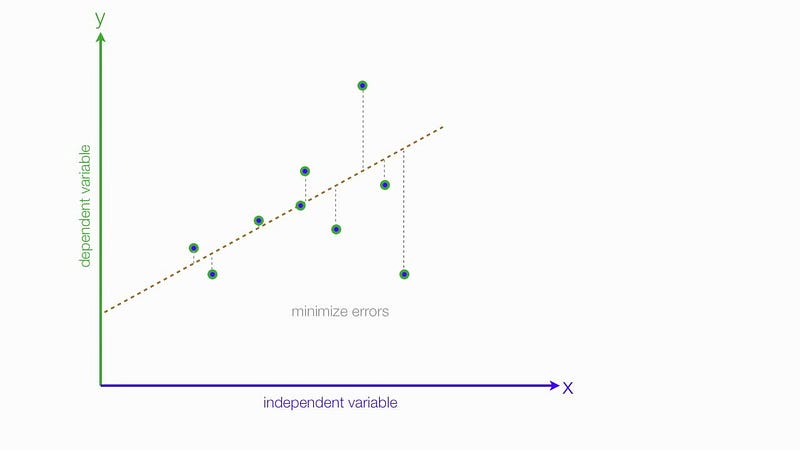
Linear Regression is used to model the relationship between two variables by fitting a linear equation to given data where one variable is explanatory variable and the other is a dependent variable.
Data for this project can be accessed here :
Let’s dive in!
Import necessary Libraries
import matplotlib.pyplot as plt
plt.style.use('ggplot')
%matplotlib inline
import numpy as np
import pandas as pd
import seaborn as sns
plt.rcParams['figure.figsize'] = (15, 10)
from mpl_toolkits.mplot3d import Axes3D
Load the Data
data = pd.read_csv('data.txt')data.info()Output —
<class 'pandas.core.frame.DataFrame'>
RangeIndex: 97 entries, 0 to 96
Data columns (total 2 columns):
Population    97 non-null float64
Profit        97 non-null float64
dtypes: float64(2)
memory usage: 1.6 KB
Visualize the Data
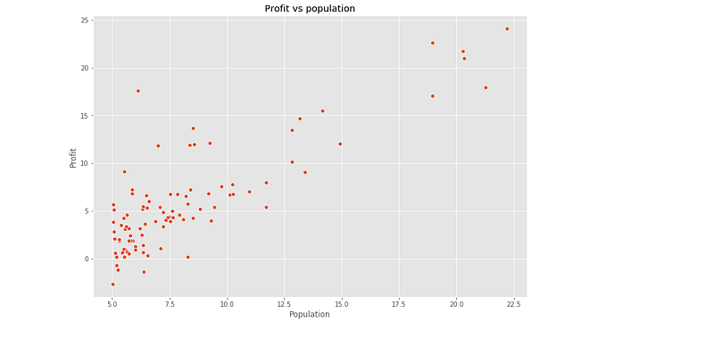
A scatterplot is used to determine the strength of the relationship between two variables in the given data.
ax=sns.scatterplot(x='Population', y = 'Profit',data=data)
ax.set_title('Profit vs population')
Output —
Compute the Cost 𝐽(𝜃)
The objective of linear regression is to minimize the cost function
def cost_function(X,y,theta):
    m=len(y)
    y_pred=X.dot(theta)
    error =( y_pred - y) **2

    return 1/(2*m) * np.sum(error)
m= data.Population.values.size
X = np.append(np.ones((m,1)),data.Population.values.reshape(m,1),axis=1)
y= data.Profit.values.reshape(m,1)
theta =np.zeros((2,1))cost_function(X,y,theta)Output —
32.072733877455676Implement Gradient Descent
Minimize the cost function 𝐽(𝜃)J(θ) by updating the below equation and repeat until convergence
def gradient_descent(X,y,theta,alpha,iterations):
    m=len(y)
    costs=[]
    for i in range(iterations):
        y_pred = X.dot(theta)
        error = np.dot(X.transpose(),(y_pred-y))
        theta -= alpha * 1/m *error
        costs.append(cost_function(X,y,theta))
return theta,coststheta, costs = gradient_descent(X,y,theta,alpha=0.01,iterations=2000)
print("h(x) = {} + {}x1".format(str(round(theta[0,0],2)),
str(round(theta[1,0],2))))Output —
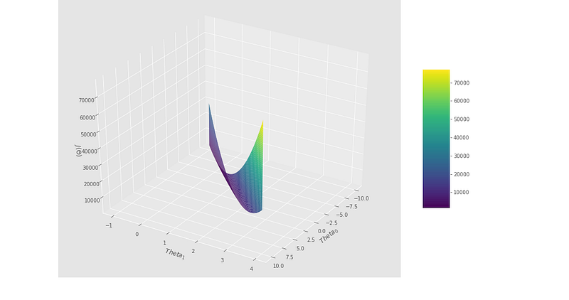
h(x) = -3.79 + 1.18x1Visualizing the Cost Function J(𝜃)
theta_0 = np.linspace(-10,10,100)
theta_1 = np.linspace(-1,4,100)
cost_values = np.zeros((len(theta_0),len(theta_1)))for i in range(len(theta_0)):
for j in range(len(theta_1)):
t=np.array([theta_0[i],theta_1[j]])
cost_values[i,j]= cost_function(X,y,t)fig = plt.figure(figsize=(15,10))ax= fig.gca(projection='3d')
surf = ax.plot_surface(theta_0,theta_1,cost_values,cmap='viridis')
fig.colorbar(surf,shrink=0.5, aspect =5)plt.xlabel('$\ Theta_0$')
plt.ylabel('$\ Theta_1$')
ax.set_zlabel('$J(\Theta)$')
ax.view_init(32,32)plt.show()Plotting the Convergence
plt.plot(costs)
plt.xlabel('Iterations')
plt.ylabel('$J(\Theta)$')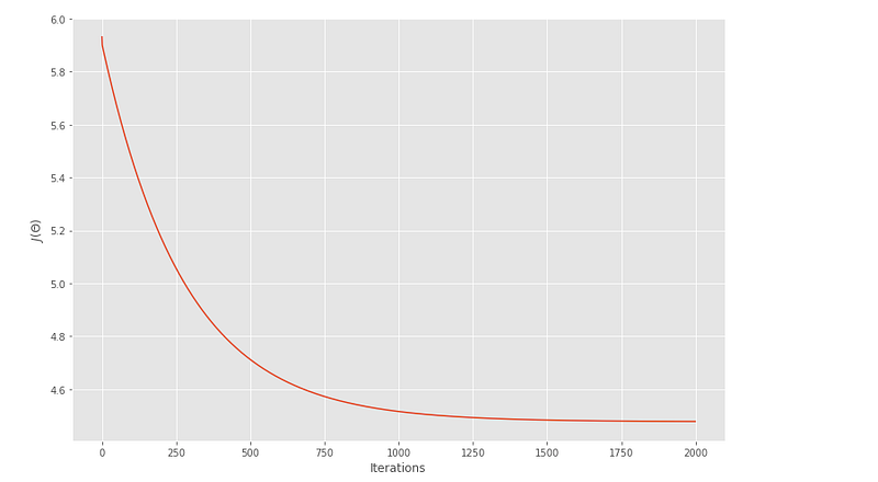
Training Data with Univariate Linear Regression Fit
theta = np.squeeze(theta)
sns.scatterplot(x='Population',y='Profit',data=data)
x_value = [x for x in range(5,25)]
y_value = [(x* theta[1] + theta[0]) for x in x_value]
sns.lineplot(x_value,y_value)plt.xlabel('Population')
plt.ylabel('Profit')
plt.title('Linear Regression Fit')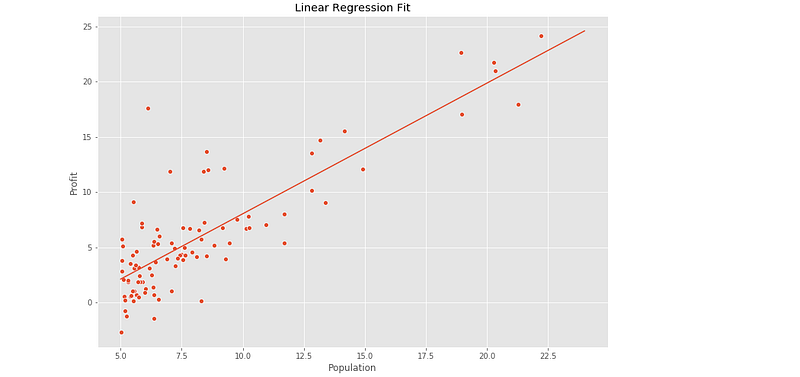
ML Regression Project 2: Coming soon
Follow and Stay tuned. Keep coding :)
For other projects, tune to —
Build Machine Learning Pipelines( With Code)
Recurrent Neural Network with Keras
Clustering Geolocation Data in Python using DBSCAN and K-Means
Facial Expression Recognition using Keras
Hyperparameter Tuning with Keras Tuner
Custom Layers in Keras
That’s it fellas. Peace out and keep coding :)
Stay Tuned and of-course let me end this post with a quote by Steve Jobs ;)
“Remembering that you are going to die is the best way I know to avoid the trap of thinking you have something to lose. You are already naked. There is no reason not to follow your heart.”


