
A Complete Introduction To Time Series Analysis (with R):: Prediction 1 → Best Predictors I
We’ve come a long way: from studying models to study time series, stationary processes such as the MA(1) and AR(1), then the Classical Decomposition Model, to Differencing and tests for stationarity. But how do we actually make predictions?? Well, as my Statistics professor said “starting linear is always a good idea”. So that’s what we will do! Be aware that in this section, we will be using some calculus and probability, so if you need a refresher on probability, check out this concept refresher that I wrote, or this excellent CS229 Probability Review document. Let’s jump into it!
Best Predictor of X_{n+h}
Recall the problem of obtaining the best linear predictor for some random variable, say Y. One could choose to solve the optimization problem
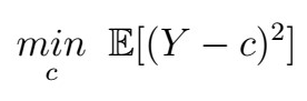
That is, we want to minimize the MSE (Mean Square Error)How can we find such a value of c? Well, from your Calculus class, you might remember that at the local minima and maxima of a function, the slope is zero, so one way is to take derivatives, set to 0, and solve for the resultant value. Furthermore, functions like the quadratic function are said to be “convex”, guaranteeing that the local minimum/maximum is also the global optimum. If some of these words don’t make much sense to you, don’t worry about it ( — Andrew Ng), as all you need to understand for now is that you can obtain the best value of c the way I described above and that that value is optimal (aka the best we can have) for convex functions. The curious souls can, however, read these slides from Standford U. on convex functions. The minimization goes as follows:
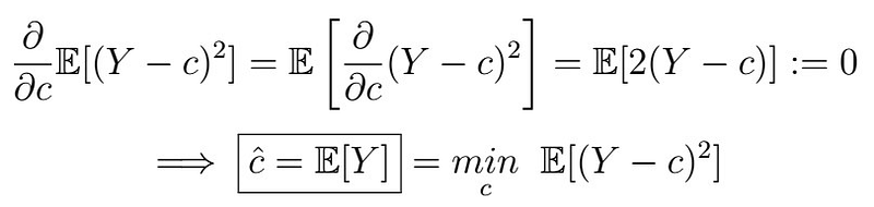
assuming we can interchange derivatives and the expectation operator (which we can do here, but once again if you are asking why we can do this, check this post ). So the best predictor is no more than the expectation of Y!!!
How can we generalize the previous to finding the best predictor of X_{n+h} given the last data point, say some function of X_{n}? What would this function be? Let’s first remember a useful tool: the Law of Total Expectation.
The Law of Total Expectation
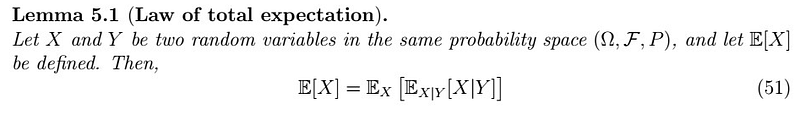
Why is this useful? Well, it adds dependence on another variable. What the L.O.E. is saying is that we can obtain the expectation of some variable that depends on another in a step way. Why does this work? Although not a general proof, here’s one for countable discrete cases:

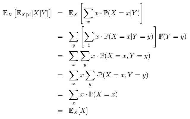
In the first line, we apply the definition of the expectation of X|Y, then we do so over the external expectation. Rearranging terms, we find that indeed, this is no more than the expectation of X alone! If you have some knowledge of measure theory, a more general proof can be found on Wikipedia (this one came from there too). Armed with this knowledge, we are now to solve our main question!
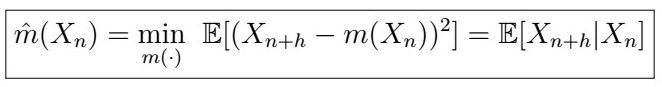
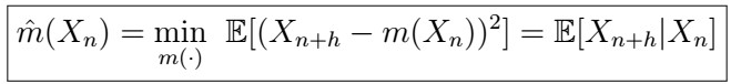
Best Predictor of X_{n+h} given X_{n}
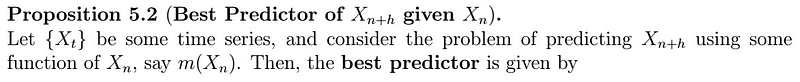
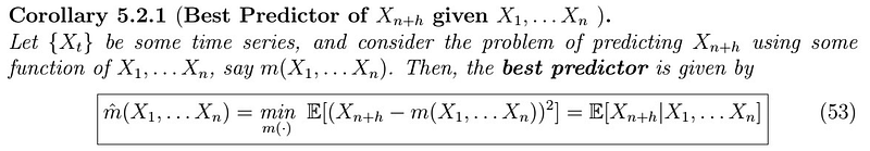
Let’s understand what this is saying:
- Suppose we consider a function m of X_{n}. How good is m()?
- Ideally, we would like such a function to be close to what we want to predict, so we consider the MSE!
- Therefore, we want to find m() that minimizes the MSE.
- It turns out that such best function is just the expectation of X_{n+h} given X_{n}!
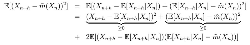
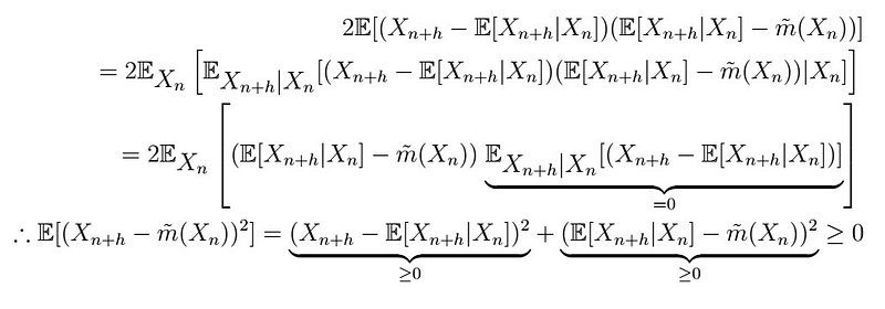
Proof
Now the L.O.E. comes in handy!!
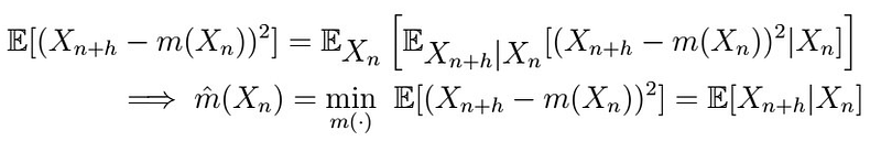
If the notation confuses you, let me explain what’s going on: the subscript indicates what kind of expectation we are taking. In the first line, we’re just applying the L.O.E. with X := X_{n} and Y := X_{n+h}. As now the inner expectation depends on X_{n}, we can treat it as a fixed constant, and therefore we are just back to the best predictor we found before!! That is, the conditional expectation you see above.
Best Predictor of X_{n+h} given X_{1},… ,X_{n}
Of course, using only one observation seems a bit.. uninformative, don’t you think so? It makes more sense to use as much data as you have or consider appropriate: ưe can extend the previous idea to a set of random variables, following exactly the same logic!
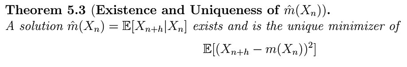
Existence and uniqueness (Optional)
Mathematicians have this obsession with showing that whatever they came up with is legitimate (which is needed, but boring to the great audience; I don’t blame you either if you do). The next section provides proof of the existence and uniqueness of such a predictor. If you don’t understand it, however, don’t worry about it. For real. I just leave this here for the curious.

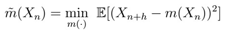
which implies that
is another minimizer of the MSE. The game we play in math for uniqueness is always of this flavor: “Assume there’s another minimum”

then show that it has to be the only one. Here it goes:
which follows by expanding out terms, simply. Therefore we have that if

Then

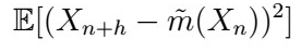
which is a contradiction as they should be equal. Indeed, it follows that
That is, the previous is just 0! Therefore, it MUST be equal! Obviously (because we love stating things that are not obvious at all), this extends to the case where we predict based on a set of observations X_{1},…, X_{n}.
Next time
Now we know that the form must of the B.L.P. must be the conditional expectation of X_{n+h} given X_{n}. But what does this actually look like? Next time we will find a model for it, using again some more calculus and statistics, as well as some of the concepts we learned before. Stay tuned!
Prediction 1 → Best Predictors II


