
A Complete Introduction To Time Series Analysis (with R):: Differencing
In the last two articles , we studied the classical decomposition model, which allows us to interpret our time series the following way:
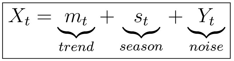
Using this powerful assumption, we can further estimate both the trend and the season, so that we have a better idea of what our series is actually “made of”. For instance, we could use the moving-average filter to estimate the trend, then estimating seasonality and carrying a classical analysis. In this article, we will learn a powerful technique to remove trend and sometimes even seasonality simultaneously: differencing. Let’s see what this is all about! For this, we will make use of two important operators: the backward shift operator and the difference operator.
Backward Shift Operator

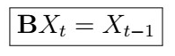
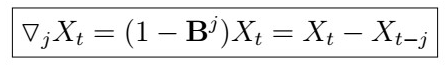
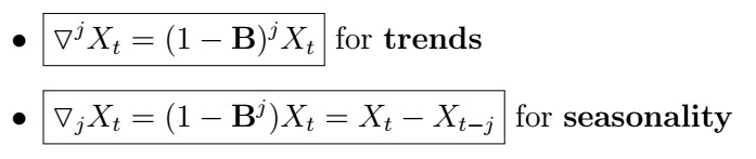
Just as it names implies, if we are given some observation at time X, the backward shift operator simply outputs the previous observation in time. Note that we can apply it more than once, which gives
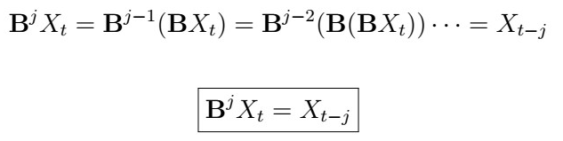
That is, applied j-times at time t, it returns back the (t-j)’th observation.
Lag-1 Difference Operator

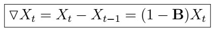
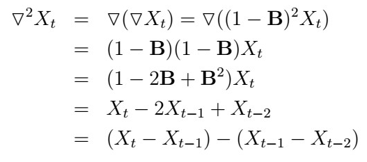
Just as its name implies, we have a difference between the current point in time and the previous one. We see that the Difference operator can also be expressed in terms of the Backward shift operator!
Difference and Lag-Difference Operators
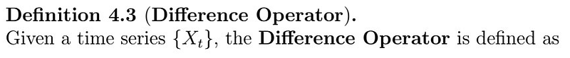
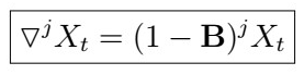
This is well-defined, as


Note that these operators are different! Although both are generalized versions of the Lag-1 difference operators, the general lag difference operator is just producing a difference between the current time point and the one j steps before, whereas the difference operator really is just applying differencing over and over. Let’s make this clear with an example:
Which is clearly not the same as
Removing trend and seasonality through differencing
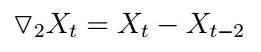
Removing trend Ok, so why do we need these? It turns out that these are very powerful in helping us remove both trend and even seasonality! How? First, suppose that we have the model
and
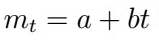
is a linear function of the trend. Then,
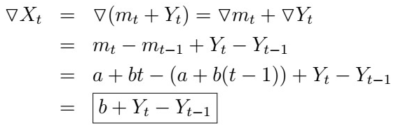

So for instance, if Yt is White Noise, differencing once will remove the linear trend and yield a stationary series. It turns out this trick also works for dealing with seasonality!
Removing seasonality
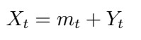
Suppose we have the classical decomposition model
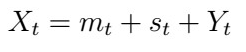
where the trend is linear and Yt is White Noise just as above. In addition, let
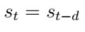
where d is the period. Then, if we apply the lag-difference operator, we obtain
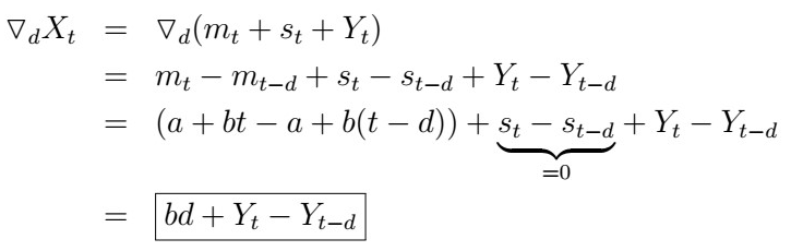
So indeed not only we removed the trend, but also the seasonality at the same time, and the residuals will be stationary so long Yt is.
When to use each difference operator?
- If there is a linear trend, we can use differencing to remove it without estimating parameters.
- Applying differencing will then yield residuals which are closer to a stationary process.
- However, note that some data is lost when applying to difference to all points (think about the boundaries! ) There is a trade-off between using different operators and predictive power!
- Although differencing can get read of trend and seasonality, in practice it is good to estimate and remove the main trend first (which has the effect of focusing on the harder-to-estimate semi-noise).
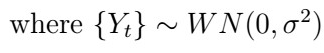
As a general rule of thumb, you might consider using
How to R
First load the necessary packages:
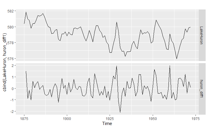
Recall the LakeHuron dataset we had previously worked with:
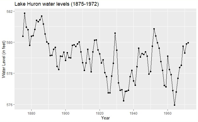
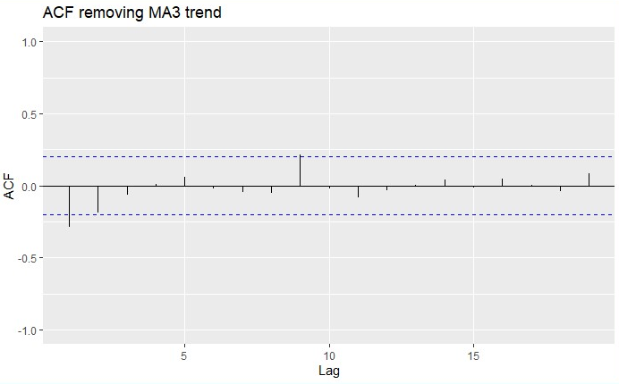
In previous articles, we had opted for estimating and removing the trend, which would in turn yield series that were closer to stationary noise. For instance, estimating and removing different trends would give the following:
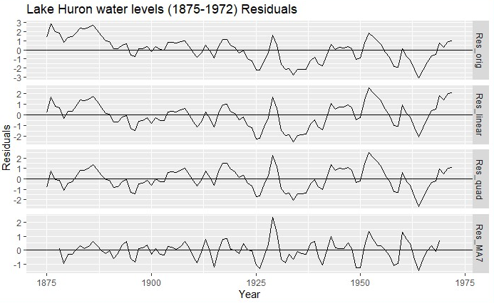
Instead of estimating the trend, we can simply apply differencing using the timeDate::diff function, yielding
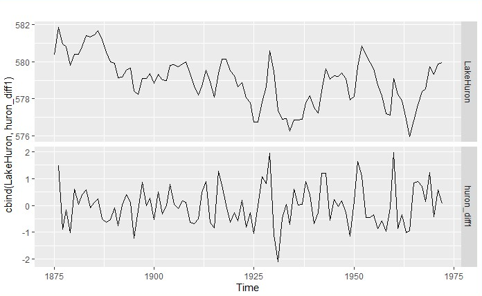
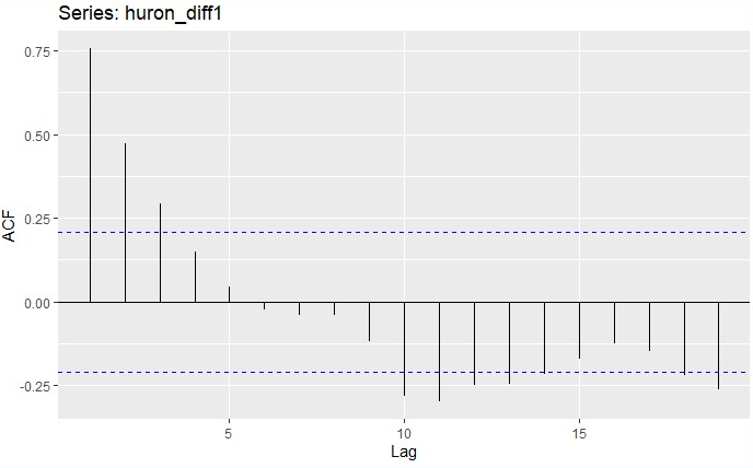
We see that the residuals indeed do not longer seem to have a clear trend and are also zero-centered. We can further inspect the ACF and PACF functions:
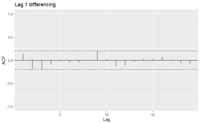
Pretty much all the lags are within bounds! That’s great! Here we only applied one lag, but what would happen if we had applied a greater lag, say 10?
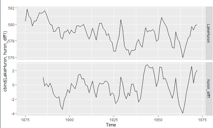
Once again, we can use ggAcf to examine the estimated ACF:
Wah! That’s a huge loss of data! If we wanted to make predictions using this data, we would have less data than before to train some models. Further, it even looks like we induced some extra-non stationarity! Indeed, there is always a trade-off between obtaining closely stationary residuals through differencing and the amount of data left. In practice, differencing is usually not that big, however.
Next time
That’s it for today! Next time, we will get a bit more mathematical and explore the properties of the autocovariance function, how to estimate autocorrelation, and more! Stay tuned, and happy learning!
Last article
Classical Decomposition Model part II


