
A Complete Introduction To Time Series Analysis (with R):: Classical Decomposition Model part I
In the last chapter, we studied the definition of stationary processes along with a couple of important examples: the IID Noise, White Noise, Random Walks, and the AR(1) and MA(1) processes, along with their respective expectations and autocovariance functions. We will now switch gears to what we saw some time ago about the trend and the seasonality, two important factors that together form the so-called classical decomposition model. In this article, we will study the classical decomposition model definition and how to estimate the trend. Let’s jump right into it!
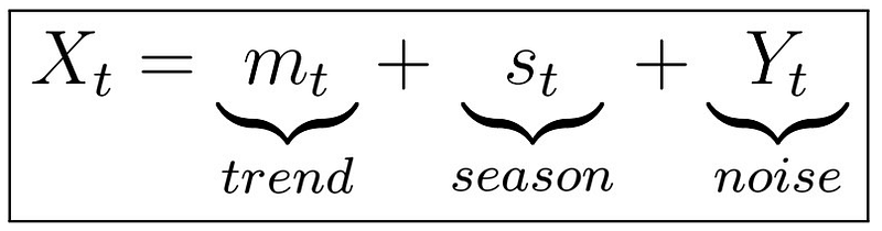
Classical Decomposition Model
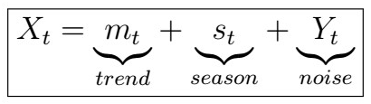
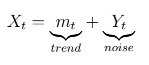
In order to perform analysis, we would like our series to be stationary, as this often helps to often fit simpler and more efficient models for prediction. The idea is very simple; consider the image above. This is saying that our model is essentially a composition of three components:
The question is, given some data, how can we know what mt or sd are? The simple answer is we don’t! However, there are techniques to perform the estimation. Let’s start with the trend.
Estimating Trends
We would like to obtain somehow accurate estimates of the trend and seasonality, without making any underlying distributional assumptions. For this reason, we use non-parametric statistics methods. Although these are more flexible, they also tend to be more subjective. In order to estimate the trend, we first assume that
, where Yt is White Noise. We will now see one of the most popular methods for this: the finite moving-average filter.
Finite Moving-Average Filter
A linear filter is defined as
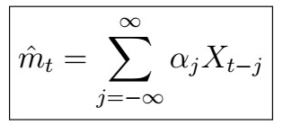
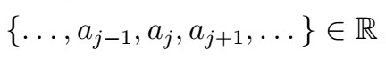
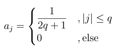
that is, this is a weighted average with real (summable) coefficients. How can we make use of this to estimate our trend? Sure, we could take an average of all the points, but let’s do something smarter. As we don’t have infinite data either, instead we use the so-called finite moving-average filter of order (2q+1), defined as follows.
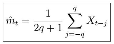
Note that the +1 is because we also sum over j=0. This is indeed a kind of linear filter, with
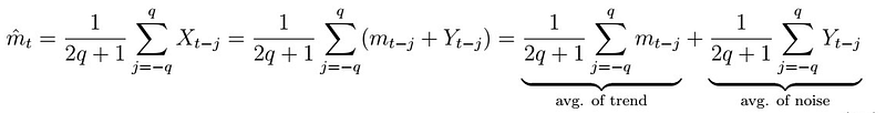
You can think of this as a “window” over the available data. which we move forward at each step, calculating “mini-averages” of a couple of points at the time. Implicitly, we are calculating both an average of the trend and of the noise at each time:
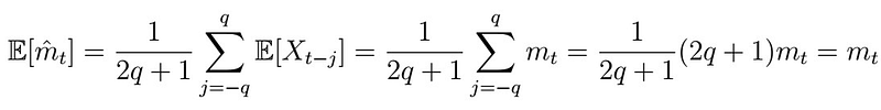
Further, this estimator is unbiased, as
Goal: We would like to shrink some of the noise, but hope not to over-shrink the trend.
How to choose q?
Ultimately, if we estimate the trend and remove it, we should have that
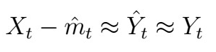
that is, the residuals should look like White Noise. How can we verify this? With ACF plots! (or stationarity tests, which we will see later).
Exponential Smoothing
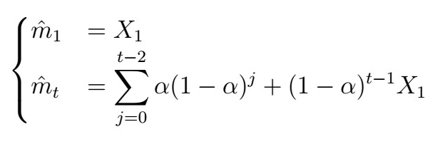
Another common technique for trend estimation in Time-Series analysis is exponential smoothing. Just as it sounds, the idea is to use some kind of exponentially weighted average, that is
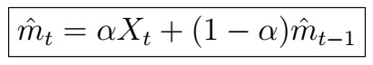
where
I will not elaborate much on this one, but if you are curious, you can check the Wikipedia page on it. In practical applications, whether you use exponential smoothing or moving-average of a relatively small order does not make much difference. Note that this is quite subjective.
Other trend estimation techniques
There are a couple of other common techniques we can use to estimate the trend, for instance, we can use
- Linear trend
- Polynomial trend
- Basis functions
- High-frequency smoothing using Fourier Series
Let’s now see a worked example of applying different trend estimations to a real dataset!
How to R
Let’s first consider the Lake Huron data from the datasets package. We start by loading the required libraries (note that some of these might not actually be necessary, but I like to include them just in case :) ):
Next, we inspect the data, which already comes in ts format.
Let’s visualize the data! We first pack the data into a tibble object, which is similar to a dataframe , and then use ggplot to plot the data.
Remember that the aes function is usually used in ggplot to pass “aesthetic properties” such as the variables themselves and sometimes the colors etc. I will not fo in-depth into explaining how it works, so if you are curious, you can check the official documentation, or use ?aes in your R studio console. Moving on, this produces the following plot:
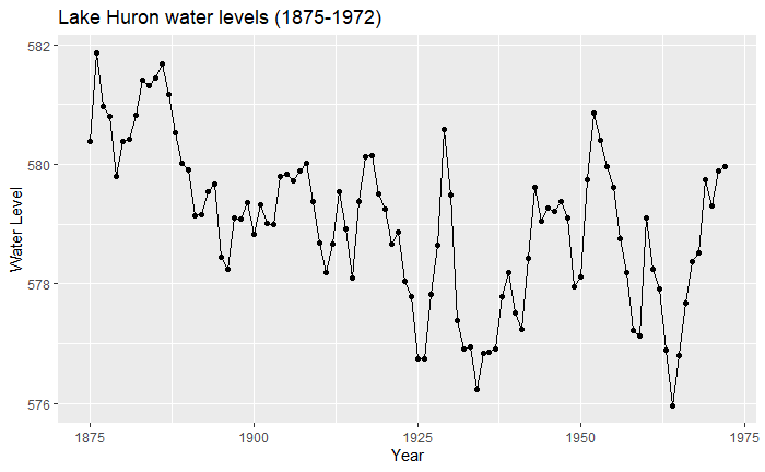
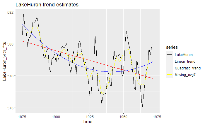
So indeed, we have some data from 1875 to 1972 on water levels for Lake Huron. What can we say about the trend? Let’s estimate a couple and see!
First, we estimate both a linear and quadratic trend using the forecast::tslm function. Next, we fit an order-7 moving average with forecast::ma . We then put all of these together and plot them, producing the following:
Pretty cool eh? However, this on its own does not tell us anything. Instead, it’s a better idea to look at the residuals, that is
Remember that after removing the trend, the result should somehow look like a stationary process or at least like a mean-zero process!
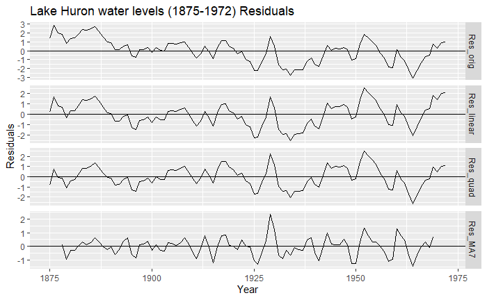
We can see that for all trends, they definitely look a lot more mean-zero than the original one, and the MA7 (order-7 moving-average) looks a bit more like White Noise than the others. You might also notice that we lost some data along the process: indeed, as we can only go over a window [-q,q], we will lose a couple of observations at the borders. We can inspect this more formally using the ACF plots we had seen before:
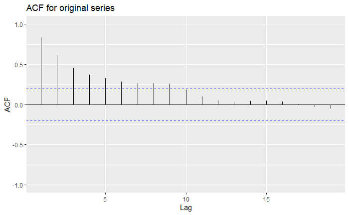
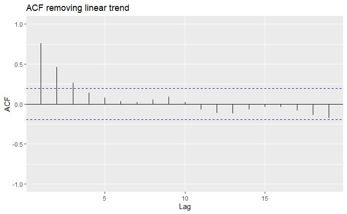
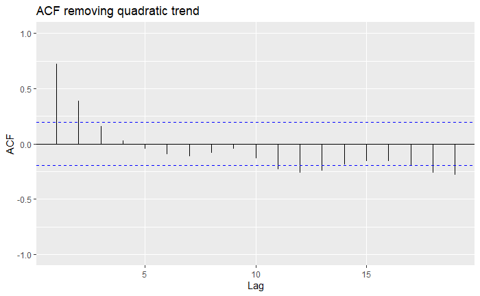
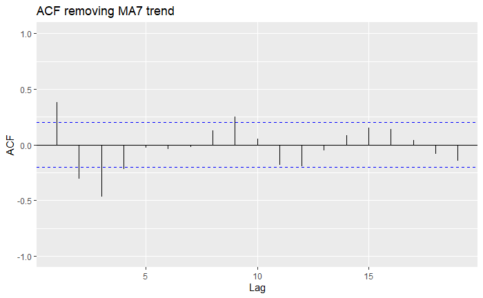
Indeed, all of our trend estimations do significantly much better than the original series, as more lags fall within the confidence bounds. However, we see that sometimes over-estimating the trend can lead to further correlation. Overall, the MA7 seems to be the best choice. The drawback is that by employing an MA filter, we sacrifice some data, and therefore, some predictive power. In the end, it is up to you to make these choices over which trend estimation to use over another!
Note: We refer to both the moving average process and the moving average filter as “MA”, but it’s clear which one is used in which context! For instance, you could use an MA5 filter to estimate an MA(1) trend (which would be zero!).
Next time
In the next article, we will see how to estimate and analyze the seasonality, so that we can get a full picture of the classical decomposition model. Stay tuned and happy learning!


