
A Complete Introduction To Time Series Analysis (with R):: MA(1)
In the last article, we explored the famous AR(1) process, and we saw that it was a mean-zero stationary process, with an ACF function that presented exponential growth (or decay, depending on the values for phi). This time, we will explore the Moving-average MA(1) process. Without anything else to say, let’s get to it.
Moving-average MA(1)
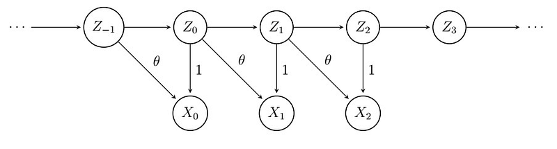
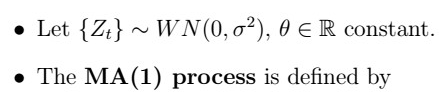
What is this saying? This says that our observations depend on present time noise, and a proportion of past noise, one step back in time. For the MA(1), we have that
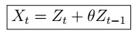
This time, it’s easy to see that it is a mean-zero process:

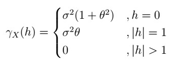
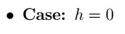
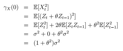
For the ACV, however, we have to consider four cases: h=0,1,-1, |h|>1. First, we have that
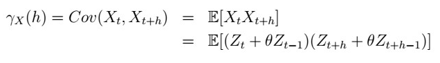
Then,
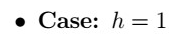
I leave it to you to verify that for the case h=-1, we obtain the exact same result. Is this a coincidence? I think not!
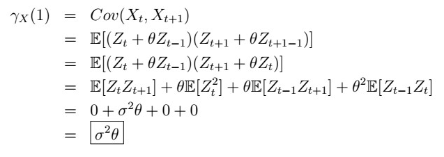
Why is the last case true? This is because
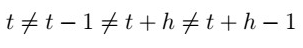
so since abs(h) > 1, these indices will never be the same and therefore the Zt’s will be uncorrelated, therefore, by the laws of expectation, each expectation of the product of two Zt’s with different indexes will become the product of their expectations, so this will just be 0.
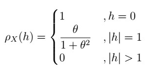
ACF of the MA(1)
If you divide each of the cases above by ACV(0), we obtain the ACF function of the MA(1) as follows:
How to R
Let’s now explore how we can produce and analyze the plots for this in R:
This time around, we only specify the ma part. Although we will not talk about this until much later, try specifying both the ar and the ma parts at the same time and see what happens! Now we obtain both of the plots for the data and the ACF:
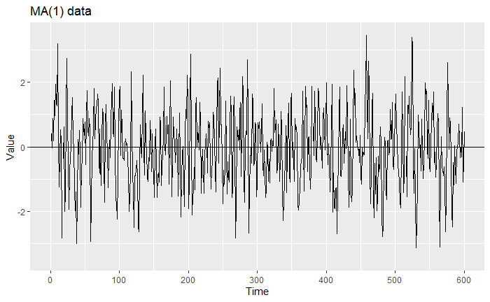
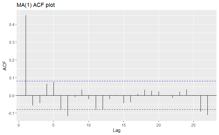
Once again, we can clearly see that the series is mean-zero and stationary. What is interesting about the MA(1), is that the first lag autocorrelation will always be really high, while all other lags will typically have small values. Compare this to the AR(1) in the previous section!
Next time
And so that wraps up the section in stationary processes. But it’s far from being over yet! Next time, we will explore a bit more in-depth the classical decomposition model, as well as some powerful techniques to estimate the trend, which we did not mention in previous articles. Stay tuned, and happy learning!


