
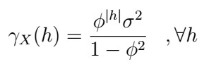
A Complete Introduction To Time Series Analysis (with R):: AR(1)
Last time, we defined a characterization of stationarity, and explored three important examples: the IID Noise, the White Noise, and Random Walks, along with how to produce and inspect their data plots and ACF plots to determine stationarity. This time, we will explore two examples of the most important processes for Time Series Analysis: the First-order autoregressive process AR(1)
First-order autoregressive process AR(1)
Let’s see the definition of the AR(1):
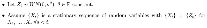
Then the AR(1) process satisfies
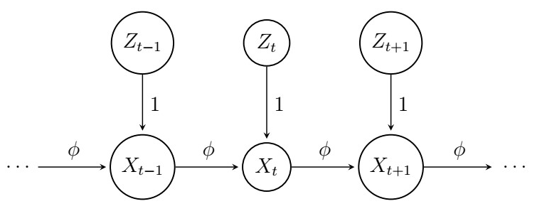
You can think of this process as follows: the value of the present observation has some dependence on the present noise and some portion of the previous time step value, but not on values further. Inspecting the mean and variance, we can easily see that

Wait, what? That’s not obvious at all! Let’s see why this is true. If we take the expectation, we have
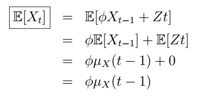
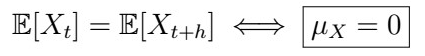
However, in order for X_t to be stationary, this can only be true if the mean is zero, that is
For the ACV (autocovariance), consider the lag h=0 (i.e. the variance)
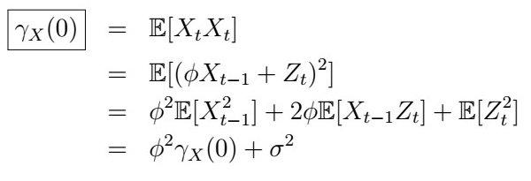
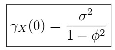
Solving for the ACV(0), we have that
When h is not 0, it follows that
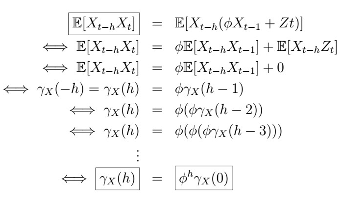
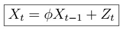
Note that sometimes we are using “+h” and others, “-h”. These are equivalent; we will see later that the ACV function is symmetric, that is, ACV(h)=ACV(-h). Plugging back what we had before,
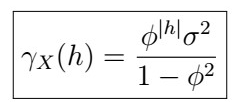
What a cool formula! Further, you can verify using the definition that the autocorrelation is given by
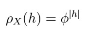
Notice something? If the absolute value of phi is more than 1, the correlation will only become worse as the lag increases! Contrarily, this tells us that if phi is less than 1 in absolute value, the autocorrelation will decrease exponentially the further the lag.
How to R
Let’s simulate some AR(1) data with phi=0.7 X:
First, we set up the true AR(1) coefficient to 0.7, then we compressed this into a list object. We set ma=NULL because we want to create an AR(1) process. Then, we pass this to thearima.sim function to generate 600 observations using the model. We can now inspect both the data plot and the ACF plot as follows:
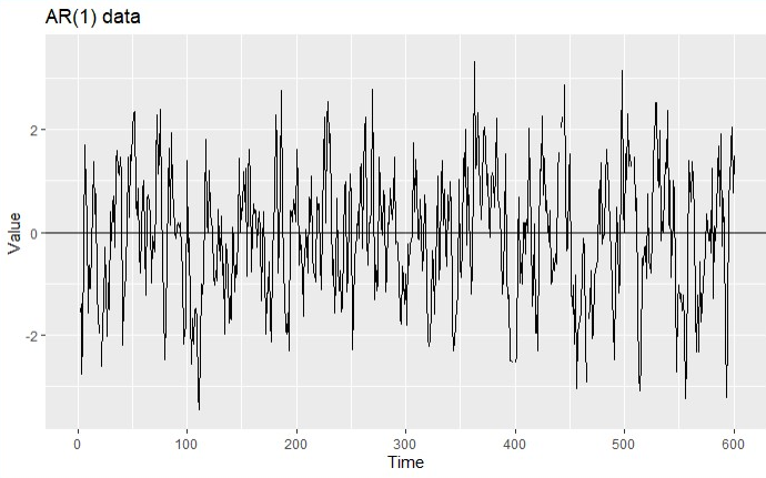
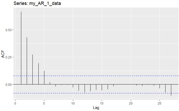
We can see that the process is indeed mean zero, and that the ACF decreases exponentially in h. Although it appears to increase a bit at lags 10 and 25, it mostly stays within the bounds.
Next time
We will continue next time with another important process: the moving average MA(1) process, along with its expectation, ACV function and cool R visualizations like these ones :)
Previous article
Main page
https://readmedium.com/a-complete-introduction-to-time-series-analysis-with-r-9882f2d44c9d


