
A Complete Introduction To Time Series Analysis (with R):: Tests for Stationarity
In the last article, we saw how we could estimate autocovariance by using a slightly modified version of the typical covariance sample estimator. Further, we saw that in reasonably large samples, this converges in distribution to a normal random variable. In this article, we will use this fact to construct some useful hypothesis tests for stationarity, to check, for instance, whether our decomposition analysis of a series in trend + seasonal component, that is, the residuals after having estimated and removed these, are correct.
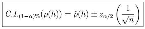
Confidence bounds for the ACF
Assuming the ACF follows an underlying normal distribution,


Lagwise Test
We can make direct use of the C.I. above to estimate whether a series is truly stationary: we know that a true stationary series should have 0 autocovariance and therefore 0 autocorrelation, so that we can employ the hypothesis
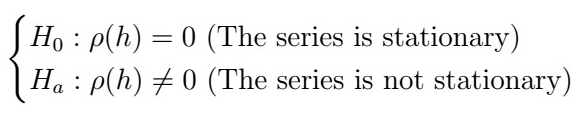
So in particular, if Ho is true, we should have that
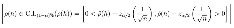
That is, the estimated confidence interval should contain the value 0 for most lags.
Portmanteau Test
This test is also quite straightforward; consider the hypothesis
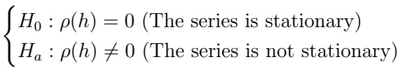
Then, using the statistic
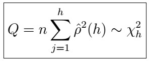
we can test the hypothesis above.
Ljung-Box Q Test
Consider the hypothesis
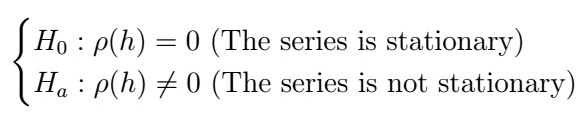
Then, using the statistic
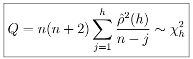
we can test the hypothesis above. Note that this is no more than a modified version of the Portmanteau Test, however, this test is more “conservative”, that is, this test is more inclined to reject H0, due to the weighting distribution.
Nonparametric tests
So far, we have seen tests that rely on normality distribution assumptions. However, there exist the so-called nonparametric tests, which do not make these assumptions, but still attempt to test whether the series is actually stationary. However, in general, these tend to be “harsher” , in that they are more likely to reject H0.
Turning points test
Consider a time series
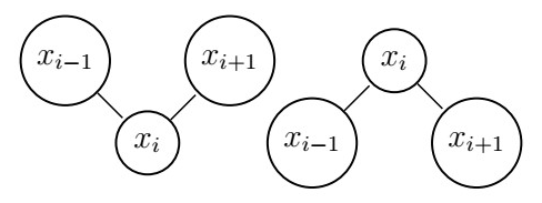
and consider any three observations from it
Then, a point xi is called a turning point if

as depicted in the figure at the beginning. Now, for an I.I.D (stationary) sequence let T be the random variable that represents the number of turning points it contains. Then, at any time t, we have that
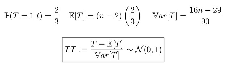
And of course, that’s entirely clear and intuitive. NOT!! WHAT THE HECK IS THIS?? Let’s think about it: the probability of a point is a turning point is 2/3 because there are 3!=6 possible permutations of three points. Out of these, only four permutations give rise to a turning point for any three points, so that the probability of a turning point is 4/6 = 2/3 at any time. For the expectation, we consider (n-2) since the edges cannot be a turning point. The variance is a lot more complicated so I won’t go over it here, but if you’re curious, you can read this stackexchange post. What is important to us is that we can use this statistic to test for stationarity, in particular, we test for an iid sequence , considering the hypotheses
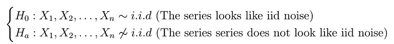

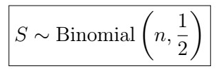
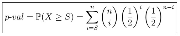
Sign Test

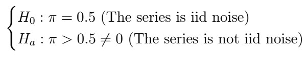
Under H0, it follows that

Other tests
Some other tests which I will not discuss in here but you will see, for instance in the R functions are :
- McLeod-Li Q test: a bootstrapping version of the Ljung-Box-Q
- Rank Test: to test for iid noise.
- Normal QQ plot: to test for distribution normality.
How to R
Great! Now we have 5 different tests to check for stationarity. Thankfully, you don’t have to manually implement these, as they already make part of R modules. Let’s first load the necessary packages
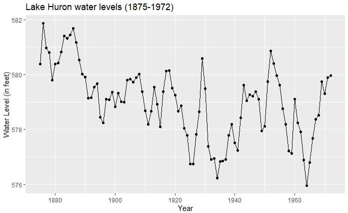
Next, let’s inspect the data by plotting the points
Next, let’s apply the tests on the raw data using the forecast::checkresiduals and the itsmr::test functions:
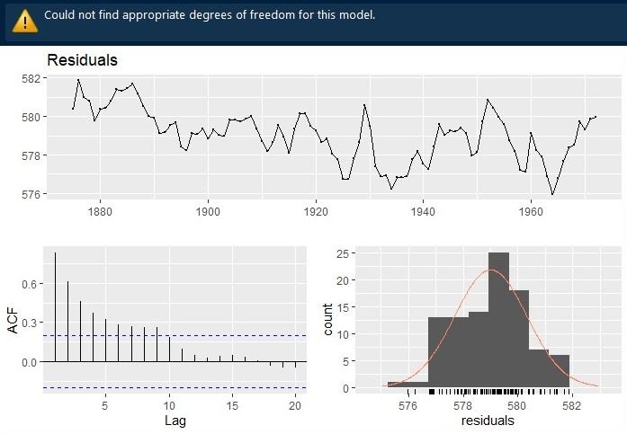
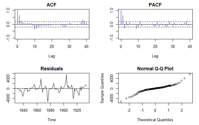
You might get the warning above; this means that the model is simply not stationary at all! So much that R could not find appropriate degrees of freedom for the Chi-square statistic. Indeed, we can observe from the ACF that most of the lag points fall off-bounds, and the underlying distribution does not look very Gaussian.
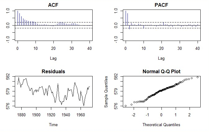
Recall that for the Ljung-Box Q test, the null hypothesis is that the series is stationary, which we clearly reject from a p-value equal to 0. Although I did not talk about the McLeod-Li Q test, the null hypothesis is the same. We also have rejection for the Turning points and Rank P test, which indicates strong non-stationarity. Let’s now difference the series and test again:
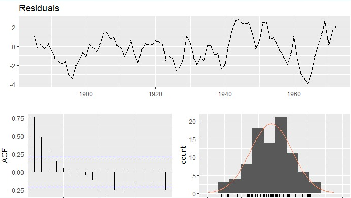
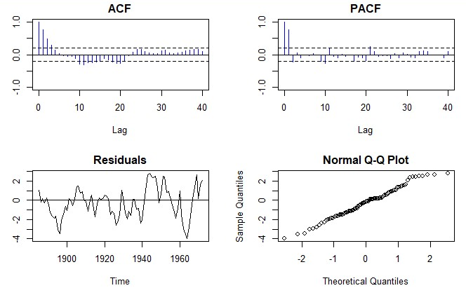
The tricky thing with these tests is that sometimes they must disagree, so it is up to the analyst or researcher to reach some meaningful conclusion, and decide what to do next. In this case, we observe that the residuals are more zero-centered, although still do not look much like actual white noise. Indeed, by inspecting the ACF and PACF, we can observe a strong correlation at the first couple of lags, which fall out of bounds, although in far less quantity than before. We do see that the empirical distribution appears to be more Gaussian, from the histogram of the empirical distribution, along with the QQ-Plot. We now see from the tests that the first three clearly reject for stationarity/iid noise (=> stationarity), but the difference sign test fails to reject the null iid hypothesis. At the 0.05 confidence, the Rank P test also fails to reject, providing some evidence for stationarity. Notice that in this example, we only applied a lag-1 difference! You could try to apply higher lag differencing or even performing a full classical decomposition analysis, as we studied in previous articles.
Next time
With this, we close the chapter on stationarity tests. Next time, we will start seeing how we can obtain the best linear predictor we can obtain, employing probability and optimization theory. Stayed tuned, and happy learning!


