
A Complete Introduction To Time Series Analysis (with R):: Estimating Autocorrelation
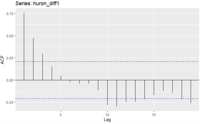
In the last article, we went over a couple of important properties of the autocovariance function, and in previous articles, we have used multiple times the ggAcf and ggPacf functions to plot the ACF and PACF respectively. But how are these actually estimated them, and how do we know that they are being correctly estimated (and hopefully not too off from the truth)? In this short article, we will explain precisely that. Let’s start!
Estimating autocovariance
Suppose that you have some time series with observed values
Then we have the following:
Sample mean
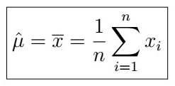
This one is probably not surprising. The interesting one is the following:
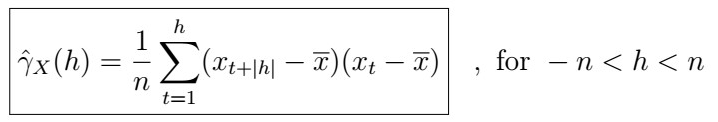
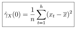
Sample autocovariance
further, this implies that
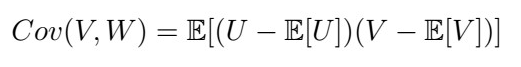
Why is this the case? First recall that the covariance between two vectors U and V is given by
When it comes to the sample version of these estimators, you can think as replacing the expectation operator by some average with the data; so, in this case, we would get
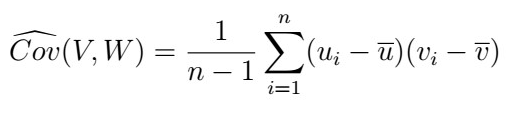
if the lowercase indexed u and v represent the random vector (observed ) components. For time series, however, both “u” and “v” come from the same data, and since we actually want to estimate the autocovariance at different lags, what we want to do instead is to “shift” the data around by the lag we wish to estimate. For instance, we can set

to estimate some lag h. This estimator is in fact biased but consistent, and it turns out this seems to work better than other unbiased estimators.
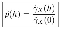
Sample autocorrelation
Just as you would expect, we have
Further, we have that this estimator follows asymptotic normality, which means that it tends to behave like a normal distribution as the sample increases. More formally,
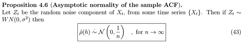
This will be very useful in the next section where we will study tests for stationarity, as several of them rely on normality assumptions. The proof of this proposition is rather hard to explain, so I won’t go over it here, but if you are curious it uses the Law of Large Numbers and Slutsky’s Theorem to show that
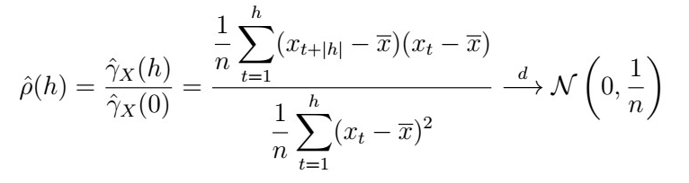
The superscript d here means that the left estimator “converges in distribution” to a normal random variable.
Next time
So that’s it for this short article! Next time we will learn a bunch of useful tests to check for stationarity of different series, using both parametric and non-parametric methods, along with illustrations in R. Stay tuned, and until next time!
Last time
Properties of the autocovariance function


