Training a Transformer Model to Predict 1-Minute Stock Prices: Tutorial with Code Samples (Part 3)

Discover How to Build an Interpretable Transformer Model for High-Frequency Stock Price Prediction, with Confidence Intervals for Risk Management.

Disclaimer: Stock price prediction is inherently uncertain, and this tutorial is intended for educational purposes only. The model and methods discussed here should not be interpreted as financial advice or relied upon for actual trading decisions. While the Temporal Fusion Transformer (TFT) model provides confidence intervals that can help assess risk, no model can fully account for the unpredictable nature of financial markets. Always conduct thorough research and consult with financial professionals before making investment decisions. This blog uses outdated data dating back to July 2024, some charts may not be accurate anymore.

Welcome back to our series on building a high-frequency stock price prediction model using the Temporal Fusion Transformer! By the end of this article, you will know how to:

Enhance your dataset with powerful technical indicators like RSI, moving averages, and support/resistance levels.
Preprocess your features and create a time series stock prices dataset that is ready to be trained on.

If you haven’t explored Parts 1 and 2, be sure to check them out to build a solid foundation in data preparation and market microstructure analysis.

This blog post is a continuation of part 2 so it assumes that the code provided there had been run prior to this. I am working on a github repo that will host all the code related to this article series and more so stay tuned.

Technical Analysis Indicators 1. Moving Averages — Moving averages serve as fundamental tools in technical analysis, helping traders identify trends by smoothing out price fluctuations. We use two types of moving averages: simple moving averages (SMA) for analyzing long-term trends and exponential moving averages (EMA) for more responsive intraday analysis.

Simple Moving Average (SMA): Calculates the unweighted mean of closing prices over a specified period, providing a clear view of the overall trend. In intraday trading, the daily SMA often acts as a crucial pivot point — if a stock in an uptrend opens below the SMA, that level typically becomes resistance when touched during the day. Conversely, for stocks in a downtrend opening above the SMA, this level tends to provide support during intraday movements.
Exponential Moving Average (EMA): Applies more weight to recent prices, making it more responsive to current market conditions. For intraday trading, the EMA effectively indicates short-term trends, functioning as support during upward trends and resistance during downward trends.

One popular strategy leveraging these moving averages is “mean reversion,” which operates on the principle that prices tend to return to their average over time. Intraday traders applying this strategy might initiate short positions when prices have sustained above the EMA for an extended period, or establish long positions when prices have remained below the EMA for a significant duration.

2. Support and Resistance Levels-Support and resistance levels represent critical price points where market psychology often leads to trend reversals or consolidation periods. These levels can be identified through historical price analysis and are valuable for both daily and intraday trading decisions. The calculation relies on fractals — local minima and maxima in the price chart.

Support Levels: Key price points where buying pressure typically increases, creating a “floor” that prevents further price decline.
Resistance Levels: Price zones where selling pressure historically intensifies, creating a “ceiling” that restricts upward movement.

Note: For detailed information on calculating these levels, please refer to my dedicated post on support and resistance analysis.

3. Relative Strength Index (RSI) The Relative Strength Index (RSI) functions as a momentum oscillator that quantifies the rate and magnitude of directional price movements. This indicator oscillates between 0 and 100, helping traders identify potential reversal points:

RSI > 70: Signals an overbought condition, suggesting a possible downward correction
RSI < 30: Indicates an oversold state, hinting at a potential upward price movement

I’ve selected these specific indicators based on my personal trading experience and their proven reliability in my strategy. However, the world of technical analysis offers numerous other powerful tools — from Bollinger Bands and MACD to Volume Profile and Market Profile. Depending on your trading style and market conditions, you might find other indicators more suitable for your model. The key is to understand each indicator’s strengths and limitations and how they complement each other in your analysis framework.

Coding Time

First I’ll define a few helper function that will make the code a little bit cleaner.

import mplfinance as mpf

def get_daily_df(minute_df, agg_dict):
    df_daily = resample_df(minute_df, "D", agg_dict)
    return df_daily

def get_hourly_df(minute_df, agg_dict):
    df_hourly = resample_df(minute_df, "H", agg_dict)
    df_hourly["hour"] = df_hourly["datetime"].dt.hour
    return df_hourly

def get_five_minute_df(minute_df, agg_dict):
    df_five_minute = resample_df(minute_df, "5T", agg_dict)
    return df_five_minute

def resample_df(df, resample_period, agg_dict):
    resampled_df = df.groupby('symbol').resample(resample_period).agg(agg_dict).dropna()
    resampled_df["symbol"] = resampled_df.index.get_level_values(0)
    resampled_df["datetime"] = resampled_df.index.get_level_values(1)
    resampled_df = resampled_df.reset_index(drop=True)
    resampled_df["date"] = resampled_df["datetime"].dt.date
    return resampled_df

def plot_bars_with_indicators(ohlc, ax, title: str, addplots=[]):
    mpf.plot(
        ohlc.rename({'open': 'Open', 'high': 'High', 'low': 'Low', 'close': 'Close'}, axis=1),
        type='candle',
        ax=ax,
        addplot=addplots,
        axtitle=title,
        ylabel='Price',
        style="yahoo"
    )

Calculate EMA and SMA:

ema_one_minute_bars = 9 * 5 # a common value for EMA lookback period is 45 minutes
sma_daily_bars = 50 # a common value for SMA lookback period on daily bars is 50 days
# Calculate the EMA and SMA
df['EMA'] = df.groupby(['symbol', 'date'])['close'].transform(lambda x: x.ewm(span=ema_one_minute_bars).mean())
df_daily = get_daily_df(df, {"close": "first"}) # we take the first close of each day to not "leak" future data into the minute bars
df_daily['SMA'] = df_daily.groupby('symbol')['close'].transform(lambda x: x.rolling(window=sma_daily_bars, min_periods=1).mean()) # very important to take the rolling moving average on the daily bars to avoid data leakage from future prices into current ones
df = df.merge(df_daily[['symbol', 'date', 'SMA']], on=['symbol', 'date'], how='left').set_index(index).rename({'SMA': 'daily_sma'})

We can plot how these averages look like on the chart, for example in Apple’s stock:

# Let's plot APPLE's daily bars with 50 day sma, and the first day of trading with 45 minute ema.
df_daily = get_daily_df(df, {"open": "first", "high": "max", "low": "min", "close": "last", "SMA": "mean"})
df_daily.set_index(pd.to_datetime(df_daily["date"]), inplace=True)
aapl_daily = df_daily[df_daily["symbol"] == "AAPL"][["open", "high", "low", "close", "SMA"]]
aapl_daily_sma = aapl_daily["SMA"]
aapl_minute = df[df["symbol"] == "AAPL"]
aapl_minute = aapl_minute[aapl_minute["date"] == df["date"].iloc[0]] # Plot the first day
aapl_minute_ema = aapl_minute["EMA"]
fig, (ax_daily, ax_minute) = plt.subplots(1, 2, figsize=(18, 8))
daily_addplot = mpf.make_addplot(aapl_daily_sma, panel=0, color='orange', ax=ax_daily)
minute_addplot = mpf.make_addplot(aapl_minute_ema, panel=0, color='orange', ax=ax_minute)
plot_bars_with_indicators(aapl_daily, ax_daily, title="AAPL Daily bars with SMA", addplots=[daily_addplot])
plot_bars_with_indicators(aapl_minute, ax_minute, title="AAPL First Day of Trading with EMA", addplots=[minute_addplot])
plt.show()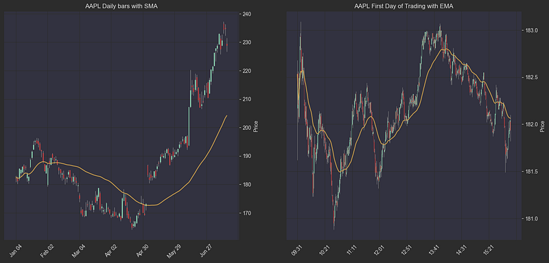

Calculating Support And Resistance Lines (Key Levels):

to see the implementation of historic_resistances and historic_supports read my dedicated post (or wait for the github repo with all the code from this series)

# resistances column holds the resistance levels (from the past) for each day
df_daily["resistances"] = df_daily.progress_apply(
    lambda x: historic_resistances(
        df_daily,
        x["symbol"],
        x["date"],
        peak_rank_w_pct=0.03, # group peaks that are within 3% of the stock price
        strong_peak_prominence_pct=0.05, # strong peaks have a prominence of at least 5%
        strong_peak_distance=10, # strong peaks are at least 10 bars away from each other
        peak_distance=5, # peaks are at least 5 bars away from each other
    ), axis=1
)
df_daily["supports"] = df_daily.progress_apply(
    lambda x: historic_supports(
        df_daily,
        x["symbol"],
        x["date"],
        trough_rank_w_pct=0.03,
        strong_trough_prominence_pct=0.05,
        strong_trough_distance=10,
        trough_distance=5,
    ), axis=1)
df_daily["resistances"] = df_daily.apply(lambda row: row["resistances"] if row["resistances"][0] > 0 else [], axis=1)
df_daily["supports"] = df_daily.apply(lambda row: row["supports"] if row["supports"][0] > 0 else [], axis=1)

We can plot a few examples to see if our key levels make sense:

def plot_with_resistances_and_supports(df, ax):
    # Create a list to hold resistance line data
    addplot = []

    last_resistances = df.iloc[-1]["resistances"]
    last_supports = df.iloc[-1]["supports"]
    for resistance in last_resistances:
        addplot.append(mpf.make_addplot([resistance] * len(df), color='red', ax=ax))
    for support in last_supports:
        addplot.append(mpf.make_addplot([support] * len(df), color='green', ax=ax))


    # Plot the candlestick chart with resistance lines
    mpf.plot(df, type='candle', addplot=addplot, style='charles',
             volume=False, ax=ax)

# plotting support and resistance for stocks
symbols = df_daily.sample(2)["symbol"].values # sample 2 stock symbols
for symbol in symbols:
    daily = df_daily[df_daily["symbol"] == symbol]
    fig, ax = plt.subplots(figsize=(18, 8))
    ax.set_title(f"{symbol} daily bars with resistance (red) and support (green) lines")
    plot_with_resistances_and_supports(daily,  ax)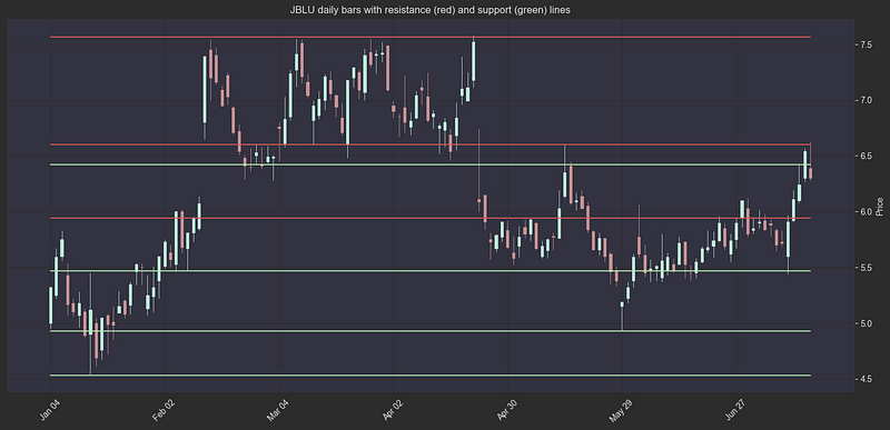

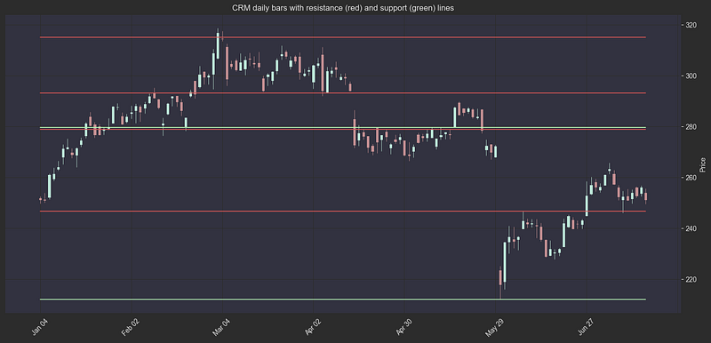
$JBLU daily bars with resistance(red) and support (green) lines

$CRM daily bars with resistance(red) and support(green) lines

Once a stock closes above a resistance or below a support line, the support price may turn into a resistance price and vice versa. Instead of treating these levels as “resistance” and “support” levels, traders call them “key levels”. Key levels are important because they are more likely to act as pivot points.

I chose to call these levels “key levels” and not distinguish between support and resistance when given as a feature to the model, you could do it differently.

df_daily["key_levels"] = df_daily.apply(lambda x: x["resistances"] + x["supports"], axis=1)
df_daily.reset_index(inplace=True, drop=True)
index = df.index
df = df.merge(df_daily[['symbol', 'date', 'key_levels']], on=['symbol', 'date'], how='left').set_index(index)
df.set_index(index, inplace=True)

Calculating RSI:

RSI is a good momentum indicator. It measures the ratio between the average green (up) bar and red (down) bar in a specified lookback window. If you are not familliar with the RSI indicator, I urge you to go read about it here. For my model, I chose the look-back window size to be 30 bars (which represents 30 minutes) because we are dealing with high-frequency prediction. However, the ideal window size might be different as I didn’t try tweaking these hyper-parameters.

This is implemented simply using the pandas-ta package

import pandas_ta as ta

WINDOW_SIZE = 30
df['RSI'] = df.groupby('symbol')['close'].transform(
  lambda x: ta.rsi(x, window=WINDOW_SIZE)
).fillna(50) # fillna 50 to represent neutral RSI

Gaps-Gaps are a common occurrence in the stock market. A gap is a break between prices on a chart that occurs when the price of a stock makes a sharp move up or down with no trading occurring in between. Gaps can be caused by a number of factors, such as news, earnings reports, or market sentiment. Traders often look for gaps as they can provide good trading opportunities. There are four types of gaps:

Common gaps: These gaps are usually small and are often filled quickly.
Breakaway gaps: These gaps occur when the price breaks out of a trading range.
Runaway gaps: These gaps occur during a strong trend and indicate that the trend is likely to continue.
Exhaustion gaps: These gaps occur at the end of a trend and signal that the trend is likely to reverse.

Gaps analysis takes into account daily gaps which are the difference between the previous day’s close and the current day’s open. Gaps are very common after earnings, as the investor’s reaction to the earnings report moves the stock in the pre-market or after-market. Stocks that open the day with a gap usually attract a lot of day traders and speculators which could make the price action even more unpredictable. We will add the day’s open gap (as log percentage of close price) as a feature to the model.

daily_df = get_daily_df(df, {
    "close": "last",
    "open": "first",
    "high": "max",
    "low": "min",
    "volume": "sum",
    "average_volume": "first"
}).reset_index() 
daily_df["previous_close"] = daily_df.groupby("symbol")["close"].shift(1).fillna(daily_df["close"])
daily_df["gap"] = np.log((daily_df["open"] - daily_df["previous_close"]) / daily_df["previous_close"])
df = df.merge(daily_df[["symbol", "date", "gap"]], on=["symbol", "date"], how="left").set_index(df_index)

For the final feature in this series, we add the hourly key levels in a similar manner to the daily key levels:

#multi time frame analysis - find support and resistance on different time frames. We will use the key levels from daily hourly and 5 minute time frames.
hourly_df = get_hourly_df(df, {"close": "last", "high": "max", "low": "min"})
hourly_df["resistances"] = hourly_df.progress_apply(
    lambda x: historic_resistances(
        df_daily,
        x["symbol"],
        x["date"],
        peak_rank_w_pct=0.005, # group peaks that are within 0.5% of the stock price
        strong_peak_prominence_pct=0.02, # strong peaks have a prominence of at least 2%
        strong_peak_distance=96, # strong peaks are at least 96 hours away from each other
        peak_distance=4, # peaks are at least 4 hours away from each other
        include_high=False
    ), axis=1
)
hourly_df["supports"] = hourly_df.progress_apply(
    lambda x: historic_supports(
        df_daily,
        x["symbol"],
        x["date"],
        trough_rank_w_pct=0.005,
        strong_trough_prominence_pct=0.02,
        strong_trough_distance=96,
        trough_distance=4,
        include_low=False
    ), axis=1
)
hourly_df["key_levels"] = hourly_df.apply(lambda x: x["resistances"] + x["supports"], axis=1)
hourly_df["date"] = pd.to_datetime(hourly_df["date"])
df["date"] = pd.to_datetime(df["date"])
df = df.merge(hourly_df[["symbol", "date", "hour" , "key_levels"]], on=["symbol", "date", "hour"], how="left", suffixes=("","_hourly")).set_index(df_index)

Data Preprocessing

Now that we have our features DataFrame, we need to preprocess it so that the model will be able to learn from it effectively. A crucial step in financial time-series modeling is converting raw price data into log returns.

Log returns are calculated as:

log_returns = np.log(price_t / price_t-1)

While I won’t delve deep into the mathematical theory here, log returns offer several key advantages over raw prices:

Stationarity: Log returns are typically more stationary than raw prices, making them more suitable for statistical modeling
Symmetry: Returns are symmetrically distributed around zero, which helps with model training
Additive Property: Returns over consecutive periods can be added together, unlike raw price ratios
Scale-Independence: Log returns allow for easier comparison across different stocks, regardless of their price levels

If you’re interested in the mathematical foundations and detailed benefits of using log returns, read this blog post.

The preprocessing phase also includes several other critical steps that we’ll implement:

Handling missing values
Feature scaling
Creating training/validation/test splits that respect time order
Sequencing our data for the TFT model

Creating Time Indices

The pytorch_forecasting package requires each row in a time-series dataset to have a unique integer index representing its position within the series. Since we have multiple time series (one per stock), we calculate this index per group:

df["month"] = df["date"].dt.month
df["day"] = df["date"].dt.day

def create_time_idx(group):
    # Use pd.factorize to create a continuous index for each symbol's time series
    group['time_idx'] = pd.factorize(group.index)[0]
    return group

df_index = df.index
df = df.groupby('symbol').apply(create_time_idx).reset_index(drop=True).set_index(df_index)

Processing Key Levels

Our key levels are currently stored as lists, which the model cannot directly process. To address this, we create separate columns for the nearest support and resistance levels, both daily and hourly:

def find_closest_resistance(row, col_name="key_levels"):
    resistances = [level for level in row[col_name] if level > row["close"]]
    if not resistances:
        return row["high"]
    return min(resistances)

def find_closest_support(row, col_name="key_levels"):
    supports = [level for level in row[col_name] if level < row["close"]]
    if not supports:
        return row["low"]
    return max(supports)

df["daily_key_level_above_current_price"] = df.apply(
    find_closest_resistance,
    axis=1
)
df["hourly_key_level_above_current_price"] = df.apply(
    find_closest_resistance,
    axis=1,
    col_name="key_levels_hourly"
)
df["daily_key_level_below_current_price"] = df.apply(
    find_closest_support,
    axis=1
)
df["hourly_key_level_below_current_price"] = df.apply(
    find_closest_support,
    axis=1,
    col_name="key_levels_hourly"
)

Feature Normalization

To normalize features across stocks with different price ranges, we transform the key levels, EMA, and SMA into percentage differences from the current price:

df["daily_key_level_above_current_price_change"] = df["daily_key_level_above_current_price"] / df["close"] - 1
df["daily_key_level_below_current_price_change"] = df["close"] / df["daily_key_level_below_current_price"] - 1
df["hourly_key_level_above_current_price_change"] = df["hourly_key_level_above_current_price"] / df["close"] - 1
df["hourly_key_level_below_current_price_change"] = df["close"] / df["hourly_key_level_below_current_price"] - 1
df["EMA_change"] = df["EMA"] / df["close"] - 1
df["SMA_change"] = df["SMA"] / df["close"] - 1

Finally, after having used the close column in its original form, I transform the close prices into log returns and scale them by 100 (for numerical stability since minute-level returns are very small), and I get rid of the open, high, low prices and replace them with close_rank. This is calculated as (close-low) / (high-low). This allows me to distill the information from the open-high-low-close bar into a single metric.

df["close_rank"] = (df["close"] - df["low"]) / (df["high"] - df["low"]) # rank of the close price in the daily range
df["log_return"] = np.log(df.groupby("symbol")["close"].pct_change() + 1) * 100 # transform close prices to log returns
df["log_return"] = df["log_return"].fillna(0) # fill NaNs with 0

Categorical features

The Temporal Fusion Transformers is built to support categorical features, so we need to convert relevant columns to the categorical pandas type:

# process categorical variables
df["month"] = df["month"].astype(str).astype("category")
df["hour"] = df["hour"].astype(str).astype("category")
df["minute"] = df["minute"].astype(str).astype("category")
df["industry"] = df["symbol"].apply(lambda x: fundamental_data[x]["industry"]).astype("category")
df["day_of_the_week"] = df["date"].dt.dayofweek.astype(str).astype("category")
df["is_earnings_day"] = df["is_earnings_day"].apply(lambda x: "yes" if x else "no").astype("category")

Data Filtering

For the purpose of this tutorial and to keep costs low, I will filter my data to contain only the 20 most traded stocks so that model training will take a reasonable amount of time and compute.

LIMIT_STOCKS = 20
top_20_average_volume_stocks = df.groupby("symbol")["average_volume"].mean().nlargest(LIMIT_STOCKS).index
df = df[df["symbol"].isin(top_20_average_volume_stocks)]
print(f"Top 20 stocks by average volume: {top_20_average_volume_stocks}")

Top 20 stocks by average volume: Index(['NVDA', 'TSLA', 'AMD', 'PLTR', 'F', 'SOFI', 'AAPL', 'RIVN', 'INTC',
   'AAL', 'PFE', 'CLSK', 'T', 'AMZN', 'CCL', 'UBER', 'MU', 'WFC', 'CMCSA',
       'GOOG'],
      dtype='object', name='symbol')

Data Split

Finally, we split our data into training, validation, and test sets:

TRAIN_PERIOD_END = "2024-06-01"
VAL_PERIOD_END = "2024-06-10"
df_train = df[df["date"] < TRAIN_PERIOD_END]
df_val = df[(df["date"] >= TRAIN_PERIOD_END) & (df["date"] < VAL_PERIOD_END)]
df_test = df[df["date"] >= VAL_PERIOD_END]
print(f"Total train rows: {len(df_train)}, Total validation rows: {len(df_val)}, Total test rows: {len(df_test)}")

Total train rows: 803394, Total validation rows: 38997, Total test rows: 199218

This split gives us 5 months of training data, 10 days for validation, and approximately 1.5 months for testing.

Temporal Fusion Transformer Setup

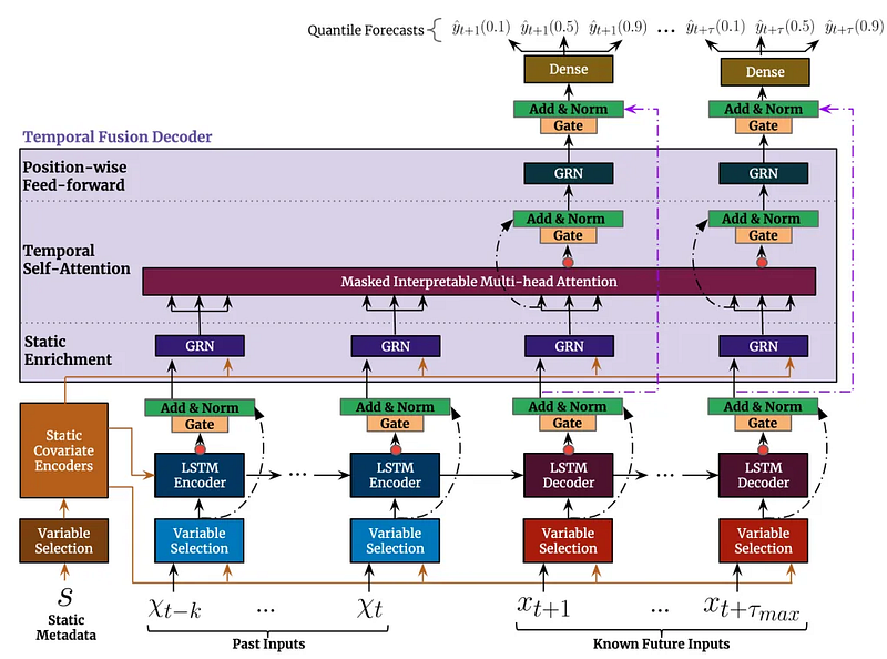
Understanding the Architecture

The Temporal Fusion Transformer (TFT) is a sophisticated deep learning architecture introduced in the paper Temporal Fusion Transformers for Interpretable Multi-horizon Time Series Forecasting by Google Research. While the paper provides a comprehensive technical overview, I recommend reading this excellent blog post that breaks down the concepts in more approachable terms.

Key Components and Capabilities

Multi-Type Variable Processing

Static Variables: Unchanging features like industry sector or company size
Time-Varying Known: Future-known features like calendar events or scheduled earnings dates
Time-Varying Unknown: Features we need to predict, like price movements and volume

2. Interpretable Multi-Head Attention Unlike traditional transformers, TFT uses a specialized attention mechanism that allows us to:

Visualize which historical time points influenced each prediction
Understand feature importance across different prediction horizons
Identify temporal patterns the model learns to recognize

3. Variable Selection Network The model automatically learns:

Which features are important for each prediction step
How feature importance changes across different forecasting horizons
When to rely more on recent versus historical data

4. Multi-Horizon Forecasting Similar to how GPT predicts the next token, TFT can:

Predict multiple time steps into the future in an auto-regressive manner
Account for varying levels of uncertainty at different time horizons
Provide quantile predictions (confidence intervals) for each forecast

Practical Applications for Stock Trading

The TFT architecture is particularly well-suited for stock prediction because:

It can process both technical indicators (time-varying) and fundamental data (static) simultaneously
The attention mechanism helps identify relevant historical patterns, similar to how traders look for chart patterns
Quantile predictions help assess risk and potential price ranges, crucial for position sizing. Could also be used for arbitrage trades.
The interpretability helps validate if the model is learning meaningful patterns rather than noise

Implementation Preview

In the next post of this series, we’ll explore how all these components work together:

How to train the model and monitor different metrics in train-time using Tensorboard
How to use built-in functionality in pytorch_forecasting to interpret the model’s predictions and attention patterns
Evaluate the model on different metrics
Implement a very basic trading strategy and backtest it

For now, let’s set up our TimeSeriesDataset, which is the foundation for training our TFT model. This dataset structure is specifically designed to handle the complex requirements of temporal data while maintaining efficient batch processing capabilities.

# if you haven't yet, run pip install pytorch_forecasting lightning
from pytorch_forecasting import Baseline, TemporalFusionTransformer, TimeSeriesDataSet
from pytorch_forecasting.data import GroupNormalizer

min_prediction_length = max_prediction_length = 20 # 20 minutes
min_encoder_length = max_encoder_length = 240 # 4 hours
training_dataset = TimeSeriesDataSet(
    df_train.reset_index(),
    time_idx="time_idx",
    target="log_return",
    group_ids=["symbol"],
    min_encoder_length=min_encoder_length, 
    max_encoder_length=max_encoder_length,
    min_prediction_length=min_prediction_length,
    max_prediction_length=max_prediction_length,
    time_varying_known_reals=[
         "time_idx", "average_volume"
    ],
    time_varying_known_categoricals=[
        "day_of_the_week", "is_earnings_day", "hour", "minute"
    ],
    time_varying_unknown_reals=[
        "close_rank", "rel_volume", "ATR", "EMA_change", "RSI", "SMA_change", "market_cap", "gap",
        "log_daily_key_level_above_current_price_change", "log_daily_key_level_below_current_price_change",
        "log_hourly_key_level_above_current_price_change", "log_hourly_key_level_below_current_price_change"
    ],
    static_categoricals=[
        "industry"
    ],
    static_reals=[
        "shares_float"
    ],
    add_relative_time_idx=True,
    add_encoder_length=False,
    target_normalizer=None # targets are already normalized
)

Let’s break down each parameter of our TimeSeriesDataSet configuration:

Core Parameters

group_ids=["symbol"]: Identifies distinct time series in our dataset. In our case, we have 20 different stocks, and each stock symbol represents an independent time series that the model will learn to predict.
time_idx="time_idx": Represents the sequential ordering of our data points. This integer index must be continuous within each stock's time series and was created during our preprocessing step to meet this requirement.
target="log_return": Specifies our prediction target, which in this case is the log returns we calculated earlier. The model will attempt to forecast this value for each step in our prediction horizon.

Sequence Length Parameters

min_encoder_length=240 and max_encoder_length=240: Sets how much historical data the model sees when making predictions. We've fixed this to exactly 4 hours (240 minutes) of data, ensuring consistent context for each prediction.
min_prediction_length=20 and max_prediction_length=20: Defines our forecast horizon of 20 minutes. We'll typically use the maximum length during actual predictions.

Feature Categorization

time_varying_known_reals=["time_idx", "average_volume"]: These are numerical features that we know in advance, even for future dates. They help the model understand temporal patterns and incorporate known future information.
time_varying_known_categoricals=["day_of_the_week", "is_earnings_day", "hour", "minute"]: These are categorical features we know in advance, such as calendar information and scheduled events. They help the model recognize periodic patterns and special market conditions.
time_varying_unknown_reals: Contains our technical indicators, market data, and normalized key levels. These are features we don't know in advance and must be predicted or estimated for future timestamps.
static_categoricals=["industry"] and static_reals=["shares_float"]: These features remain constant for each stock throughout the time series. They help the model adjust its predictions based on fundamental characteristics of each stock.

Advanced Features

add_relative_time_idx=True: Adds normalized time index features that help the model understand relative temporal positions within sequences.
add_encoder_length=False: We've disabled adding sequence length as a feature since we're using fixed-length sequences of 240 minutes.

This configuration creates a dataset that feeds our model 4 hours of historical data to predict the next 20 minutes of returns. The pytorch_forecasting package automatically handles all the necessary scaling and normalization of features, making it easier to focus on the model architecture and trading strategy rather than data preprocessing. This is one of the key advantages of using this package — it abstracts away all the time series data preparation under the hood, ensuring our features are properly scaled and normalized for optimal model training.

Wrapping Up

In this post, we’ve covered the essential groundwork for building a stock price prediction model using the Temporal Fusion Transformer. We started with fundamental technical indicators like Moving Averages, Support/Resistance levels, and RSI, transformed our raw price data into meaningful features, and set up a sophisticated dataset structure using pytorch_forecasting. The TFT architecture is particularly exciting for this task because it can handle multiple types of features while providing interpretable predictions with confidence intervals.

Coming Up in Part 4: Training Our Market Prediction Model

Now that we have our feature engineering pipeline and dataset structure in place, we’re ready to bring our trading strategy to life with machine learning. In Part 4, we’ll:

Train the Temporal Fusion Transformer on our multi-feature dataset
Analyze the model’s attention patterns to understand what it learns from the market
Interpret prediction confidence intervals for risk management
Develop a simple trading strategy based on the model’s outputs
Backtest our approach

If you’ve enjoyed this deep dive into feature engineering and want to see how we transform market data into actionable trading signals, be sure to follow me for Part 4. Clap for this story if you found it helpful, or support my work through the PayPal link below!