How to Calculate Support and Resistance Levels Using Python: A Step-by-Step Guide

Support and resistance levels help traders make better decisions by highlighting key price levels where trends might reverse. Understanding these levels can aid in identifying optimal entry and exit points for trades.

AAPL Candlestick Chart With Support And Resistance Levels

Disclaimer: I do not provide investment advice and I am not a qualified licensed investment advisor.

TICKERS MENTIONED IN THIS ARTICLE: $AAPL $AVGO

Support and resistance lines are key concepts in technical analysis used by traders to identify potential turning points in the price movement of a stock or other asset. A support line represents a price level where a downtrend tends to pause or reverse due to a concentration of buying interest. Conversely, a resistance line indicates a level where an uptrend might halt or reverse because of selling pressure. These levels are used by traders to make decisions about entering or exiting trades, estimating risk, and predicting future price movements.

In this short blog post I will show you an algorithm that I implemented in Python that calculates these lines on any time-frame, whether it’s 5 minute bars or 1-day bars.

Implementation

First install the required packages.

pip install yahooquery pandas scipy mplfinance

Then import them.

import yahooquery as yq
import pandas as pd
import scipy as sp
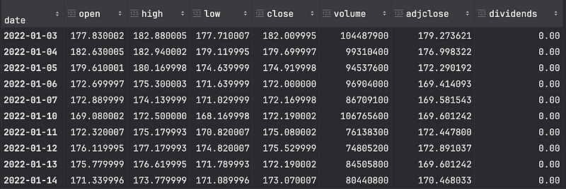
import mplfinance as mpf

Load historical daily bars into a dataframe. We will take Apple’s stock for this tutorial.

bars = yq.Ticker('AAPL').history(start='2022-01-01', interval='1d').reset_index(level=0, drop=True)

This gives a data frame with daily bars starting from 01/01/2020 until today, it looks like this:

Visualizing Historical Price Data

Before we identify support and resistance levels, let’s visualize the historical price data for better context. We will plot the closing price of the stock over time.

bars.index = pd.to_datetime(bars.index)
mpf.plot(bars, type='candle', style='charles', title='(AAPL) Candlestick Chart', volume=True)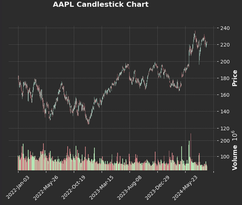

Identifying Peaks and Troughs with SciPy

The find_peaks function from the scipy.signal module detects local maxima (peaks) in data. In the context of stock prices, these peaks can serve as potential resistance levels. Let’s take a look at the key parameters we use:

• distance: Specifies the minimum number of data points between consecutive peaks. This helps avoid detecting too many peaks too close to each other.

• prominence: A peak’s prominence represents how much it stands out from the surrounding data. The higher the prominence, the more significant the peak.

Strong Peaks

In my approach, I treat “strong” and “weak” peaks separately. I define “strong” peaks as those with high prominence and greater separation (distance), as well as significant price levels like the 52-week high. This is how we find them using find_peaks:

# Define the distance between strong peaks (in days).
strong_peak_distance = 60

# Define the prominence (how high the peaks are compared to their surroundings).
strong_peak_prominence = 20

# Find the strong peaks in the 'high' price data
strong_peaks, _ = sp.signal.find_peaks(
  bars['high'],
  distance=strong_peak_distance,
  prominence=strong_peak_prominence
)

# Extract the corresponding high values of the strong peaks
strong_peaks_values = bars.iloc[strong_peaks]["high"].values.tolist()

# Include the yearly high as an additional strong peak
yearly_high = bars["high"].iloc[-252:].max()
strong_peaks_values.append(yearly_high)

This code identifies significant resistance levels based on price prominence and separation. The strong_peaks_values list contains the high prices of the strong peaks, as well as the 52-week high:

[176.14999389648438,
 198.22999572753906,
 199.6199951171875,
 237.22999572753906,
 237.22999572753906]

As you can see, some of these values are very close to each other. That’s perfectly fine — later on, we’ll merge peaks that are too close to ensure cleaner resistance levels.

Here’s how you can plot the resistance lines we found so far using mplfinance (mpf). We’ll plot the candlestick chart along with the identified strong peaks as resistance lines.

# Create a list of horizontal lines to plot as resistance levels
add_plot = [mpf.make_addplot(np.full(bars.shape[0], resistance), color='r', linestyle='--') for resistance in strong_peaks_values]

# Plot the candlestick chart with resistance lines
mpf.plot(
    bars, 
    type='candle', 
    style='charles', 
    title='AAPL Candlestick Chart with Strong Resistance Lines',
    volume=True, 
    addplot=add_plot
)

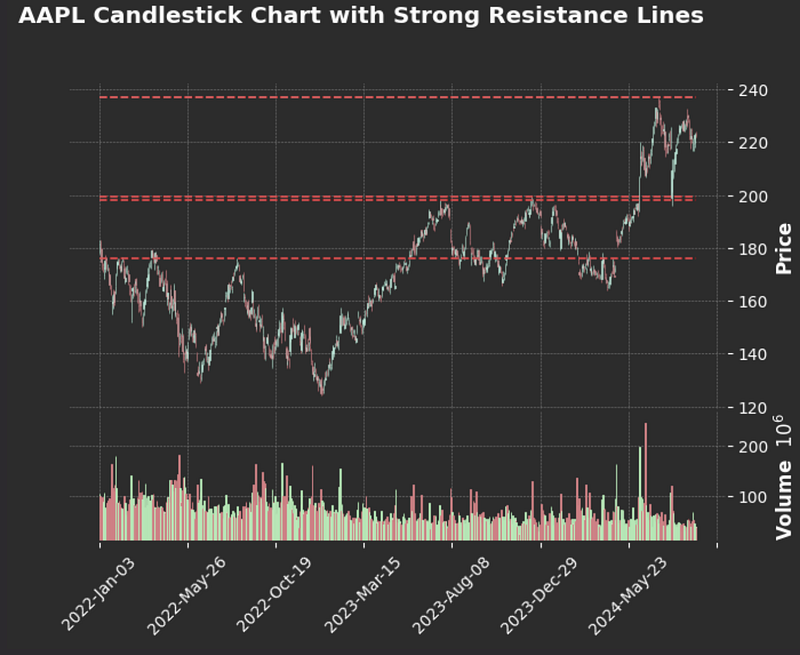
AAPL Candlestick Chart With Strong Resistance Lines

This gives a solid representation of long-term resistance levels. However, swing traders often focus on shorter-term price movements, looking for more frequent peaks and resistance points. This is where general peaks come into play, providing insights into shorter-term trends and resistances.

General Peaks

I define general peaks as those with weaker prominence and shorter distance compared to strong peaks. However, for a price level to qualify as a “general peak,” the stock must reach and be rejected from that level multiple times.

To achieve this, I set both a minimum width and a minimum rank threshold. These thresholds help group weaker peaks into bins, merging nearby peaks that are too close to one another. If a peak level reaches the minimum rank (i.e., the stock price has been rejected at that level enough times), it is added to my list of resistance levels.

This approach helps identify shorter-term resistance levels, which are particularly useful for swing traders who focus on smaller price movements over shorter time periods. These general peaks complement the strong peaks to provide a more comprehensive view of resistance levels in the stock’s price history.

# Define the shorter distance between general peaks (in days)
# This controls how far apart peaks need to be to be considered separate.
peak_distance = 5

# Define the width (vertical distance) where peaks within this range will be grouped together.
# If the high prices of two peaks are closer than this value, they will be merged into a single resistance level.
peak_rank_width = 2

# Define the threshold for how many times the stock has to reject a level
# Before it becomes a resistance level
resistance_min_pivot_rank = 3

# Find general peaks in the stock's 'high' prices based on the defined distance between them.
# The peaks variable will store the indices of the high points in the 'high' price data.
peaks, _ = sp.signal.find_peaks(bars['high'], distance=peak_distance)

# Initialize a dictionary to track the rank of each peak
peak_to_rank = {peak: 0 for peak in peaks}

# Loop through all general peaks to compare their proximity and rank them
for i, current_peak in enumerate(peaks):
    # Get the current peak's high price
    current_high = bars.iloc[current_peak]["high"]
    
    # Compare the current peak with previous peaks to calculate rank based on proximity
    for previous_peak in peaks[:i]:
        if abs(current_high - bars.iloc[previous_peak]["high"]) <= peak_rank_width:
            # Increase rank if the current peak is close to a previous peak
            peak_to_rank[current_peak] += 1

# Initialize the list of resistance levels with the strong peaks already identified.
resistances = strong_peaks_values

# Now, go through each general peak and add it to the resistance list if its rank meets the minimum threshold.
for peak, rank in peak_to_rank.items():
    # If the peak's rank is greater than or equal to the resistance_min_pivot_rank, 
    # it means this peak level has been rejected enough times to be considered a resistance level.
    if rank >= resistance_min_pivot_rank:
        # Append the peak's high price to the resistances list, adding a small offset (1e-3) 
        # to avoid floating-point precision issues during the comparison.
        resistances.append(bars.iloc[peak]["high"] + 1e-3)

# Sort the list of resistance levels so that they are in ascending order.
resistances.sort()

# Initialize a list to hold bins of resistance levels that are close to each other.
resistance_bins = []

# Start the first bin with the first resistance level.
current_bin = [resistances[0]]

# Loop through the sorted resistance levels.
for r in resistances:
    # If the difference between the current resistance level and the last one in the current bin 
    # is smaller than a certain threshold (defined by peak_rank_w_pct), add it to the current bin.
    if r - current_bin[-1] < peak_rank_width:
        current_bin.append(r)
    else:
        # If the current resistance level is far enough from the last one, close the current bin
        # and start a new one.
        resistance_bins.append(current_bin)
        current_bin = [r]

# Append the last bin.
resistance_bins.append(current_bin)

# For each bin, calculate the average of the resistances within that bin.
# This will produce a clean list of resistance levels where nearby peaks have been merged.
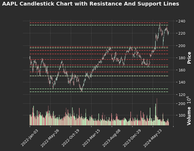
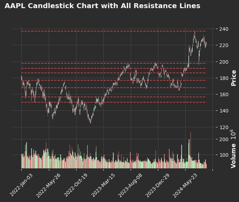
resistances = [np.mean(bin) for bin in resistance_bins]

Here is the same chart with all the combined resistance levels:

Troughs (Support Levels)

The cool thing about finding support levels, is that it can be done exactly just like resistance levels, except we pass in the negative values of our lows:

troughs, _ = sp.signal.find_peaks(-bars['low'], distance=peak_distance)

Everything else is quite the same, except use the low values of the bars instead of the highs. I will leave the implementation to you, but here is how the chart looks like with both resistances and supports:

Conclusion

In this post, we explored how to calculate and visualize support and resistance levels using Python. By leveraging libraries like yahooquery, scipy, and mplfinance, we identified both long-term and short-term price levels where a stock like Apple ($AAPL) may face significant buying or selling pressure.

This method of separating strong and general peaks provides a flexible approach that can be adapted to different time frames and stocks, making it valuable for traders and investors alike. Whether you’re looking for key reversal points or short-term trading opportunities, understanding support and resistance levels can help improve decision-making and refine your trading strategy.

Thanks for Reading!

Thank you for taking the time to read this post! If you found it helpful, feel free to follow me for more content. I’m planning to release a multi-episode guide on training a transformer model on minute-level stock bars, so stay tuned for that series!