Summary

This context discusses the application of the Extended Kalman Filter (EKF) for nonlinear systems, which is a modification of the standard Kalman Filter to handle nonlinear transition and observation models.

Abstract

The context begins by introducing the concept of nonlinear systems and the need for a filter that can handle such systems. It then explains the background of the Extended Kalman Filter (EKF), which is a modification of the standard Kalman Filter to handle nonlinear transition and observation models. The EKF uses the First-Order Taylor Approximate to linearize nonlinear functions. The context then provides the code for implementing the EKF in Python, which involves updating the input such that the transition and observation models are no longer constant but functions that return a constant given input. The context concludes by providing an example of the application of the EKF to a nonlinear system and the results obtained.

Bullet points

The context discusses the application of the Extended Kalman Filter (EKF) for nonlinear systems.
The EKF is a modification of the standard Kalman Filter to handle nonlinear transition and observation models.
The EKF uses the First-Order Taylor Approximate to linearize nonlinear functions.
The context provides the code for implementing the EKF in Python.
The context concludes by providing an example of the application of the EKF to a nonlinear system and the results obtained.

Timeseries Methods: Kalman Filter from Scratch Part 4

Introduction

So far, we focused on linear transition and observation matrix. However, there are times when we are likely to believe that nonlinear models will better describe the system. Given Kalman Filter is the best linear filter an option is for us to linearize the nonlinearity.

Background

We can linearize nonlinear function using First-Order Taylor Approximate. Details can be found here. We are stating that for a nonlinear and differentiable function f

Thus, for the nonlinear transition model F and nonlinear observation model H at each step of update we will compute the partial derivative of each state variable evaluated at the prior estimate. Everything else remain the same as the linear counterpart, except the F and H at each update step is no longer constant. They become time dependent.

Code

From the original class we kalman_filter class we created in here, we just need to update the input such that F and H are no longer constant, but functions return a constant given input. Note that given B and u are arbitrary predetermined control vector whether or not they are linear is not of concern here.

Below is the updated class. Please note the structure did not change. The L and M deals with non-additive noise component. it will be ignored in the case of additive noise components. Alternatively, you can use the override methods from FilterPy package’s ExtendedKalmanFilter. Since it only allows for nonlinear in the transition matrix.

class extend_kalman_filter:
    def __init__(self, x_init, transition_model, observation_model, F_partial, Q, R, H_partial,
                 L_partial, M_partial
                 , B=None, u=None,  sd=np.array([[0]])):
        self.x_init = x_init
        self.F = F_partial
        self.Q = Q
        self.R = R
        self.H = H_partial
        self.L = L_partial
        self.M = M_partial
        self.transition_model = transition_model
        self.observation_model = observation_model
        self.X_post = self.x_init
        self.P_post = sd
        self.X_prior = None
        self.P_prior = None
        if B is not None and u is not None:
            self.B = B
            self.u = u
        else:
            self.B = np.array([[0]])
            self.u = np.array([[0]])

        self.mean = np.zeros_like(self.x_init)
        self.covar = np.zeros((sd.shape[0], sd.shape[1]))

    def fit(self, data, num_state=1, fit_step=None):
        self.num_state = num_state
        fit_step = fit_step if fit_step is not None and fit_step < data.shape[1] else data.shape[1]
        for i in range(fit_step):
            z_k = data[:, i]
            # predict
            self._predict(self.X_post, self.P_post)
            self._update(z_k)
            # update
            self.mean = np.append(self.mean, self.X_post, axis=1)
            self.covar = np.append(self.covar, self.P_post, axis=0)

    def _predict(self, X_post, P_post):
        self.F_current = self.F(X_post)
        self.L_current = self.L(X_post)
        self.X_prior = self.transition_model(X_post, self.B, self.u)
        self.X_prior = self.X_prior.reshape(X_post.shape)
        self.P_prior = np.dot(np.dot(self.F_current, P_post), self.F_current.T) + \
                       np.dot(np.dot(self.L_current,self.Q),self.L_current.T)

    def _update(self, observation):
        self.H_current = self.H(self.X_prior)
        self.M_current = self.M(self.X_prior)
        resid = observation - self.observation_model(self.X_prior)
        S_k = np.dot(np.dot(self.H_current, self.P_prior), self.H_current.T) + \
              np.dot(np.dot(self.M_current,self.R),self.M_current)

        K_k = np.dot(np.dot(self.P_prior, self.H_current.T), np.linalg.inv(S_k))
        self.X_post = self.X_prior + np.dot(K_k, resid).reshape(self.X_prior.shape)

        self.P_post = np.dot(np.eye(self.num_state) - np.dot(K_k, self.H_current), self.P_prior)

    def new_observation(self, observation):
        num_new_obs = observation.shape(self.num_state)
        for i in range(num_new_obs):
            obs = observation[:,i]
            self._predict(self.X_post, self.P_post)
            self._update(self, obs)

    def predict(self, n_step=1, B_new=None, u_new = None):
        ## assume no control
        pred_array = np.zeros((self.H_current.shape[0], n_step))
        X_cur = self.X_post
        for i in range(n_step):
            X_new = self.transition_model(X_cur)
            Y_new = self.observation_model(X_new)
            pred_array[:,i] = Y_new
            X_cur = X_new

        return pred_array

Application

Let us assume that the model is defined as below

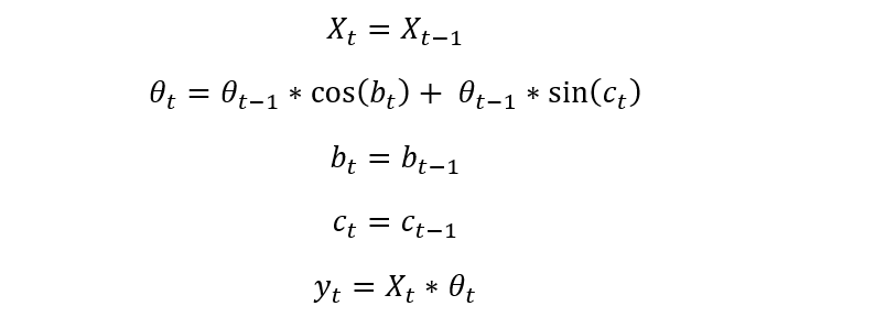
In code it looks like this

    x_init = np.ones((4, 1))
    def x_new(inputs, *args):
        return_mat = np.zeros_like(inputs)
        return_mat[0] = inputs[0]
        return_mat[1] = -inputs[1]*np.cos(inputs[2]) - inputs[3] * np.sin(inputs[2])
        return_mat[2] = inputs[2]
        return_mat[3] = inputs[3]
        return return_mat

    def y_new(inputs):
        return inputs[0] + inputs[1]*inputs[0]

    def F_partial(inputs):
        return_mat = np.eye(inputs.shape[0])
        return_mat[1,1:] = [-np.cos(inputs[2]), inputs[1]*np.sin(inputs[2])-inputs[3]*np.cos(inputs[2]),
                            -np.sin(inputs[2])]
        return return_mat

    def H_partial(inputs):
        return np.array([inputs[1,0],inputs[0,0],0,0]).reshape(1,4)


    def L_partial(inputs):
        return np.eye(inputs.shape[0])

    def M_partial(inputs):
        return 1

    Q = np.eye(4)
    R = 1
    kf = extend_kalman_filter(x_init, x_new, y_new, F_partial, Q, R, H_partial,
                 L_partial, M_partial
                 , B=None, u=None,  sd=Q)
    n_train = int(len(data) * 0.9)
    n_test = len(data) - n_train
    kf.fit(observation[:,:n_train], 4, n_train)
    fittedvalues = kf.get_observation()
    pred_ = kf.predict(n_test)

To make it a fair comparison with the linear version, a linear version with exactly 3 states is chosen （as opposed to the 6 states from the previous two posts are multistate and multidimensional）

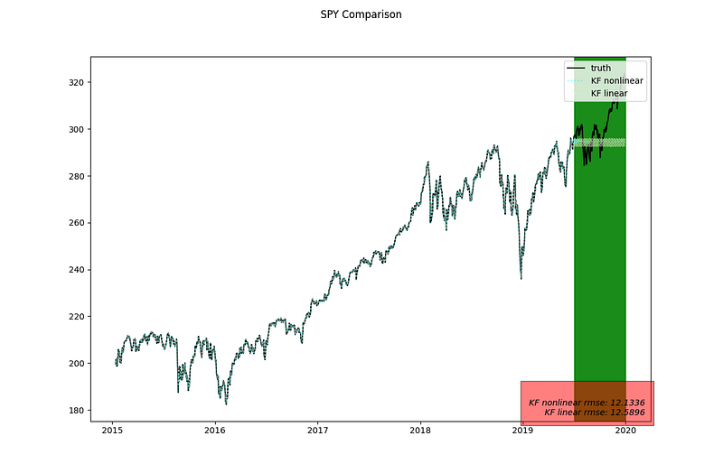
Results

This is the complete plot over the training and testing periods.

This is the result for just the testing period

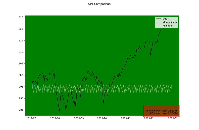
What we can notice that in the first few time-step post training it has more of a variance period to period and then flattens out to an average for time periods further out.

There is an alternative option to deal with nonlinear setup, it is the unscented kalman filter. We will explore this in future post.

Thank you for reading. Please follow and subscribe if you are interested in more posts on time series analysis.