Timeseries Methods: Kalman Filter from scratch in Python — Part 3

This post will continue to explore other usage of Kalman Filter methods, mainly as an alternative to do multivariate forecast. Other option includes Vector Autoregressive (VAR). This post will not go into details on VAR, but rather provide an alternative on modeling multi-dimensional output when a transition process is known. It is important to know that when using Kalman Filter both the relationship between unobserved variable and the observed output is known (or have a reasonable assumption) as well as how the unobserved variable transitions to the next timer period is known (assumed). In addition, all the modelling done so far has a linear assumption, both the transition process and the observation process are linear.

Introduction

For those unfamiliar with Vector Autoregressive models, you can find detailed information from wiki. In python the statsmodel package has built-in functions for VAR, detailed usage can be found in documentation.

In short, VAR is used if we believe that the observed variables interact together. This paper proposes a PC-VAR which has been applied to model many economic series. A quick example is interest rates. Interest rates are highly correlated and there are numerous series (from overnight all the way to 30 year rates), but it can be easily reduced to 3 dimensions using principal component analysis (PCA). The first 3 components of interest rate is well defined as “level”, “slope” and “curvature”, which would explain 95%+ of the variance in interest rate. We would then apply VAR on these principal components, solve for the coefficients simultaneously.

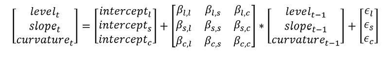
Regarding PC-VAR, there is transformation to turn the raw interest rates into principal components, apply VAR on the principal components to run prediction and then transform the principal components back into interest rates. Please note in practice, there is significant difficulty for the model to predict level （which accounts for over 50% of the variance in interest rate).

Multidimensional Kalman Filter

In this post we will be analyzing the SP500 time series along with 2-year interest rate.

The transition matrix is designed as such that

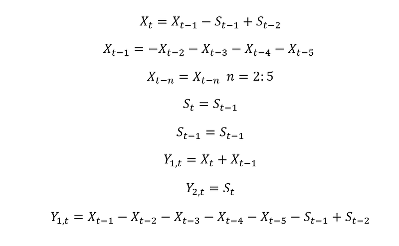
Here is the code: Note the treasury rate is from US Department of Treasury.

    n_train = int(len(data) * 0.9)
    n_test = len(data) - n_train
    result_set = {}
    graph_text = ""
    filter_input = np.concatenate([sp_return.T, interest_rate], axis=1)

    kf = KalmanFilter(transition_matrices=[1], observation_matrices=[1],
                      transition_covariance=np.array([[1]]), observation_covariance=1,
                      n_dim_obs=1)
    kf_mean, filtered_std = kf.filter(filter_input[:n_train,0])
    kf_pred = np.array([1]) * np.power(np.array([1]), np.arange(n_test-1)) * kf_mean[-1]
    result_set = {'kf-1 state': np.append(kf_mean[5:], kf_pred.reshape(-1,1))}
    graph_text = "kf-1 rmse: " + "{:.4f}".format(rmse(filter_input[n_train:,0],kf_pred))


    n_season = 5
    F = np.zeros((n_season + 1, n_season + 1))
    F[0,0] = 1
    F[1, 1:-1] = [-1.0] * (n_season - 1)
    F[2:,1:-1] = np.eye(n_season - 1)
    H = np.array([1, 1, 0, 0, 0, 0])
    P_init = np.eye(n_season + 1) * 0
    P_init[:2,:2] = np.eye(1) * Q
    kf = KalmanFilter(transition_matrices=F, observation_matrices=H,
                      transition_covariance=P_init, observation_covariance=1,
                      n_dim_obs=1)
    kf_1, filtered_std = kf.filter(filter_input[:n_train,0])
    filtered_obs = kf_1.dot(H)
    filtered_pred = forecast_kf(n_test-1, kf_1[-1], F, H.reshape(1,-1))
    graph_text += "\nkf_5 rmse: " + "{:.4f}".format(rmse(filter_input[n_train:,0],filtered_pred))
    result_set['kf_5_2'] = np.append(filtered_obs[5:], filtered_pred.reshape(-1,1))

    n_int=2
    F = np.zeros((n_season + 1 + n_int, n_season + 1 + n_int))
    F[0,0] = 1
    F[0,-2:] = [-1, 1]
    F[1, 1:n_season] = [-1.0] * (n_season - 1)
    F[2:n_season+1,1:n_season] = np.eye(n_season - 1)
    F[-2,-2] = 1
    F[-1,-2] = 1
    H = np.array([[1, 1, 0, 0, 0, 0, 0, 0],[0,0,0,0,0,0,1,0]])
    P_init = np.eye(n_season + 1 + n_int) * 0
    P_init[:2,:2] = np.eye(2) * Q
    P_init[-2:,-2:] = np.eye(2) * Q
    R = np.eye(2) * R
    X_0 = np.zeros(n_season + 1 + n_int)
    kf = KalmanFilter(transition_matrices=F, observation_matrices=H,
                      transition_covariance=P_init, observation_covariance=R,
                      initial_state_mean=X_0, initial_state_covariance=P_init,
                      n_dim_state=8
                      )
    mean_, std_ = kf.filter(filter_input[:n_train,:])


    filtered_pred = forecast_kf(n_test-1, mean_[-1], F, H)
    fitted_value = np.dot(mean_,H.T)
    result_set['SPY Kalman with Treasury'] = np.append(fitted_value.T[0,5:], filtered_pred[0,:])
    graph_text += "\nSPY Kalman with Treasury rmse: " + "{:.4f}".format(rmse(filter_input[n_train:,0], filtered_pred[0,:]))
    ## VAR
    model = VAR(filter_input[:n_train,:])
    results = model.fit(1)
    filtered_pred = results.forecast(filter_input[n_train-1:n_train,:], n_test-1)
    result_set['SPY VAR(1)'] = np.append(results.fittedvalues[4:,0], filtered_pred[:,0])
    graph_text += "\nSPY VAR(1) rmse: " + "{:.4f}".format(rmse(filter_input[n_train:,0], filtered_pred[:,0]))

    results = model.fit(5)
    filtered_pred = results.forecast(filter_input[n_train - 5:n_train, :], n_test - 1)
    result_set['SPY VAR(5)'] = np.append(results.fittedvalues[:, 0], filtered_pred[:, 0])
    graph_text += "\nSPY VAR(5) rmse: " + "{:.4f}".format(rmse(filter_input[n_train:, 0], filtered_pred[:, 0]))

The result is as follow, please note in the plot below it only looks at the SP500 return prediction, ignores the result for the interest rate prediction to be inline with the other posts. The power of the model is that it predicts both series.

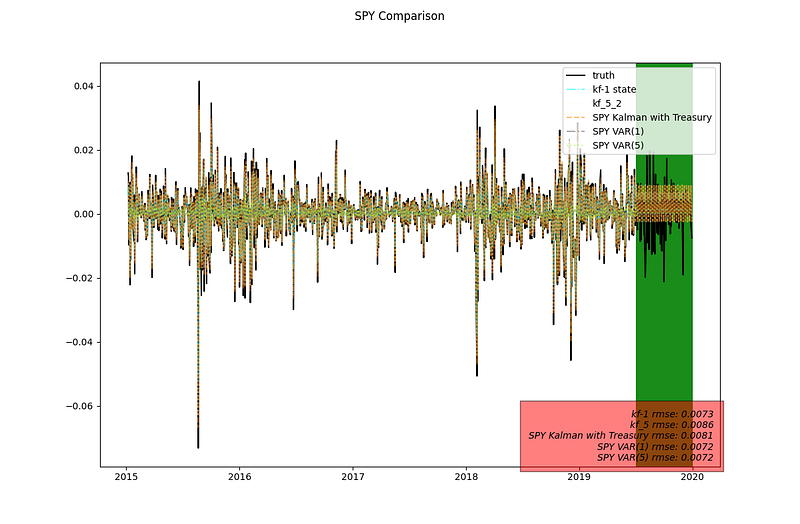
magnifying over the green testing period

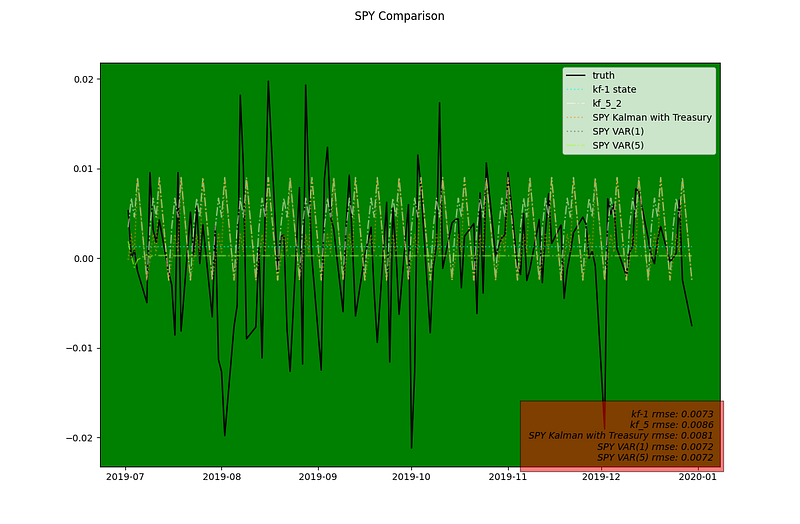
There is a slight difference between the Kalman Filter with cyclic term from last post （named kf_5 here and kf_5_2 previously, mostly the second hump is less pronounced with the inclusion of Treasury Rate.

Conclusion

Looking closely into it, we noticed that that although there is a slight decrease in RMSE with the inclusion of treasury, the directional accuracy drops slightly. We could improve the model set by taking the inspiration from the PC-VAR model to include additional interest rate series （first applying PCA to reduce dimensionality） and / or we could include other equity return (DJ) or series such as volatility index.

Things to Consider

So far, we have made some strong assumptions (linearlity) and no unknown parameter in the transition and observation model. In many use cases, these are not true. In the future posts we will explore how to deal with nonlinear transition model and how to estimate the parameters.

Please follow and subscribe if you are interest in future posts on the subject.